Nondestructive detection of saline-alkali stress in wheat (Triticum aestivum L.) seedlings via fusion technology | Plant Methods

Plant material and experimental design

The experimental wheat material used in this research was Jimai 22, which is widely planted in China. The experimental samples were screened in terms of similar size, quality, with no surface damage. Before the experiment, the wheat was disinfected with 75% alcohol for 5 min and rinsed 3 times with distilled water. Wheat seeds were treated with different stress treatments from the germination stage. After 5 days of germination, the wheat was transplanted into a black hydroponics box with different stress treatment solutions for culture. On the basis of previous studies, the concentration with high stress and low mortality was selected, and the concentration suitable for saline-alkali stress identification in wheat seedling stage was 100 mmol/L [20]. Three experimental treatments were set as control (CK, distilled water), A [100 mmol/L neutral salt (NaCl: Na₂SO₄ = 9:1, pH = 6.68)], and B [100 mmol/L alkaline salt (NaHCO₃: Na₂CO₃ = 9:1, pH = 8.9)], and there were four replications for each treatment. The wheat seedlings were incubated in an MGC Series Intelligent Light incubator (MGC-450BP-2L, Shanghai Yiheng Scientific Instruments Co., Ltd., Shanghai, China) at 25 ± 1 °C with 80% relative humidity and 12 h/12 h alternating light and dark period. Relevant indicators of different treatment groups of wheat were collected every 2 days.

T2 acquisition and processing

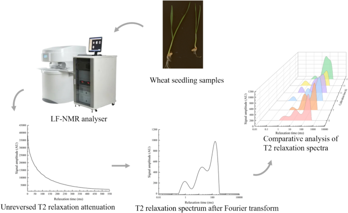
The LF-NMR instrument (AniMR, Shanghai Newmark Electronic Technology Co., Ltd., Shanghai, China) was used to collect the transverse relaxation time (T2) of LF-NMR. The basic parameters of the instrument were as follows: Magnetic field intensity: (0.25 ± 0.05) t; Resonance frequency: 8.5–12.8 MHz; Magnetic field uniformity: less than 10 ppm (φ60 mm × 100 mm); Magnet temperature: 32℃; Probe coil diameter: 15 mm. The Carr–Purcell–Meiboom–Gill (CPMG) sequence pulse sequence in the NMR spectrum analysis software was used to determine the T2 of the sample. According to the previous test results [7, 15], the main sampling parameters were set as follows: 90° hard pulse width (P1) = 8 μs; 180° hard pulse width (P2) = 12 μs; Sampling frequency(SW) = 200 kHz; Analog gain (RG1) = 43.5 db; Digital gain (DRG1) = 3; Number of signal sampling points (TD) = 907,218; Repeated sampling times (NS) = 16; Waiting time for repeated sampling (TW) = 5000 μs; Echo number (NECH) = 18,000.

The LF-NMR spectrum analysis is a quantitative analysis and detection method using the spectral signal obtained by the Fourier transform of NMR signal. The CPMG collected from the experiment was imported into NMR spectrum inversion software, and the Simultaneous Iterative Reconstruction Technique (SIRT) was used for inversion operation. T2 was obtained after inversion. The inversion parameters were set as follows: minimum relaxation time: 0.01 ms; Maximum relaxation time: 10,000; Number of participating inversion points: 200; Number of iterations: 10,000. In order to eliminate the influence of inconsistent initial quality of test samples on the test results, all signal amplitude data were normalized, and then the data were imported into SPSS 23 for one-way analysis of variance. The OriginPro 2022 was used for drawing in this paper. During the test, the collection of CPMG was repeated three times, and the average value was taken. CPMG of wheat seedlings were collected on the 5th, 7th, 9th, 11th and 15th day of seedling growth. The instrument would be calibrated before each collection, and the water on the sample surface would be wiped gently with absorbent paper to avoid moisture affecting the results (Fig. 1).

T2 relaxation data acquisition and analysis process

Multispectral image acquisition and processing

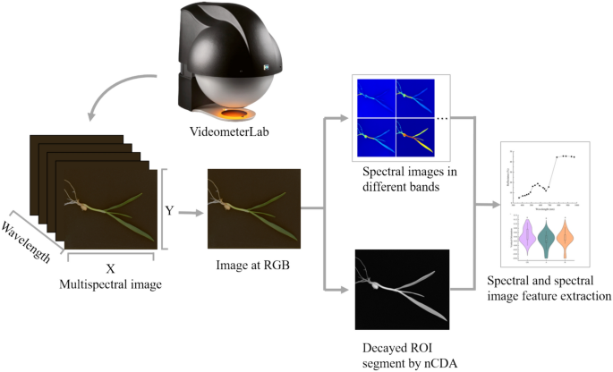
The multispectral images of all wheat seedling samples were taken by a VideometerLab 4 instrument (Videometer A/S, DK-2700 Herlev, Hørsholm 12B, 3.sal, Denmark). The instrument consists of a sphere containing 19 light emitting diodes in the wavelengths 375, 405, 435, 450, 470, 505, 525, 570, 590, 630, 645, 660, 700, 780, 850, 870, 890, 940 and 970 nm. All images were acquired in one sequence, with a resolution of 4096 × 3000 pixels, and a pixel size of 0.03 mm per pixel. Surface reflectance was recorded by the involvement of a standard monochrome charge coupled device chip [45]. Before acquiring multispectral images, the system was fully calibrated radiometrically and geometrically by using three successive plates: a white one for reflectance correction, a dark one for background correction and a doted one for geometric pixel position aligning calibration, followed by a light setup calibration [15, 23].

The multispectral images obtained contained not only wheat seedlings but also some other interference, such as the background board and surrounding debris (Fig. 2). Therefore, it was necessary to remove these objects before extracting the spectral information of individual wheat seedlings. The images were processed using Videometerlab software version 3.22. Background removal in images of complete wheat seedlings was achieved through Normalized Canonical Discriminant Analysis (nCDA), and the seedlings were segmented using a simple threshold. Morphological traits and main spectral features were then extracted from the segmented wheat seedling images. The morphological traits were divided into shape features, color features, and binary features. The shape features included BetaShape_a, BetaShape_b, Compactness Circle, Compactness Ellipse, Vertical Orientation, and Vertical Skewness; color features included CIELab_A, CIELab_B, and CIELab_L; binary features included Area, Length, and Width. The interpretation of morphological shapes was listed in the supplementary file: Supplementary material.

Multispectral data acquisition and analysis process

The extracted spectral features represented the average intensity of reflected light at each single wavelength, calculated from all the wheat seedling pixels in the images.

Determination of germination index

The 450 wheat seeds were selected and evenly divided into 9 groups. Each kind of solution (CK, A, and B) was used to cultivate 3 groups of seeds individually. Before the experiment, the wheat was disinfected with 75% alcohol for 5 min and then rinsed three times with distilled water. The wheat seeds were placed on germination paper that had been moistened with an adequate amount of the corresponding solution, ensuring that both the paper and the seeds were sufficiently dampened. The germination paper was changed daily, and the cultivation environment was maintained as described in “Plant material and experimental design”. The number of germinated seeds in each group was recorded daily until the 7th day. The germination rate, germination potential, germination index, and average germination time of the wheat were calculated, with the respective formulas shown below [28].

Detection model and performance evaluation

Prediction model of moisture signal quantity

Four regression models including Gradient Boosting Regression Tree (GBRT), Support Vector Machine (SVM), Kernel Partial Least Squares Regression (KPLSR) and Back Propagation Neural Network (BPNN) were established to predict the moisture signal of wheat seedlings under saline-alkali stress using MSI data. Before establishing the quantitative model analysis, the correlation analysis between MSI data and signal amplitude A was established by using Spearman and Kendall algorithm, and the multispectral data with high correlation was selected as the input variable of the model.

For the performance evaluation of the regression model, six evaluation criteria were selected: determination coefficient of training set (R2_c), corrected root mean square error (RMSEC), prediction determination coefficient (R2p), prediction root mean square error (RMSEP), training time (s), and predicting speed (obs/s). Wherein, R2 measures the proportion of variation explained by the model in the total variation, and the value range is from 0 to 1; The closer the R² value is to 1, the more variation in the data the model explains, indicating better model fitting. In addition, RMSE measures the prediction error of the model on the training set; The smaller the value of RMSE, the better the performance of the model on the training set. The training time and speed reflect the efficiency of the model in practical application. The calculation formula of R2 and RMSE were as follows.

where i is the data point, n is the number of data points, \(y_{i}\) is the actual value, \(\hat{y}_{i}\) is the predicted value, and \(\overline{y}\) the average value of the actual value.

Classification prediction model

In this study, we discussed the application effect of K-Nearest Neighbor (KNN) and Gaussian-Naïve Bayes (GNB) combined with fivefold cross validation method in the classification and prediction model of salt and alkali stress in wheat seedlings. We used three different datasets: MSI datasets, LF-NMR datasets, and fusion datasets of MSI and LF-NMR. At present, KNN and GNB have shown satisfactory results in the field of classification [10].

The prediction performance of the classification model was evaluated by four key indicators: Precision, Recall, Accuracy and F1-score. Precision is the ratio of true positive data to all predicted positive data, indicating the classifier’s ability to avoid labeling negative cases as positive. Recall is the ratio of true positive predictions to all actual positive data, indicating the classifier’s ability to identify all positive samples. Accuracy is the percentage of samples that are correctly classified by the model, reflecting the overall effectiveness of the classifier on the given dataset. The F1-score is a metric that combines the trade-off between Precision and Recall, providing a single number that reflects the effectiveness of a classifier, particularly in the presence of rare categories. It is calculated as the harmonic mean of Precision and Recall [7, 21]. The four equations of the evaluating indicators were:

where TP, TN, FN, and FP are for true positive, true negative, false negative, and false positive, respectively.