Proposal for a classification system of radiographic bone changes after cervical disc replacement | Journal of Orthopaedic Surgery and Research

Development of the classification system

A classification system in the present study was iteratively developed over a 12-month period, during which the co-authors convened as a panel to collaboratively evaluate serial radiographs of cTDRs and previous classification studies for cTDR [12, 18, 19, 28] and total joint replacement [13, 14]. The panel consisted of six investigators, including four experienced cTDR surgeons (AK, FP, TL, GA), an experienced large joint orthopaedic surgeon (JJ), and a clinical researcher (SMK) with experience in TDR revision and assessment of bony changes in radiographs around large total joint replacements. Because our goal was to assess radiographic changes over time, and cTDRs routinely exhibit gaps or radiolucent lines immediately after implantation that gradually fill in over time, assessments were not made based on an isolated set of radiographs. This approach was consistent with best practices of assessing bony changes around hip and knee total joints. We initially considered the use of anterior–posterior (AP) radiographs as part of the classification system, however we found that the APs of the cTDR cases available to us were more variable in terms of readability and angle of the incident beam, making evaluation of the interface more difficult. Hence, we relied on lateral radiographs as the basis for our classification system. Radiographs from 34 patients representing 44 implants from 7 implant systems were reviewed to aid in the development of the classification system, specifically for the purpose of identifying and agreeing on bone change descriptions and important implant considerations. The radiographs were sourced from the spine surgeon coauthors’ recent cTDR cases, in particular those with exemplary imaging.

The classification protocol for assessing radiographic changes was based on lateral plain radiographs of the cervical spine, dividing the vertebral body into three sections, anterior, middle, posterior, approximating sections as shown in Fig. 1. Attention was focused on characterizing changes around both the superior and inferior endplates in these three sections. Note that these figures are artists renderings of radiographs to convey the particular observed anatomy. Example of radiographs from patients used in the study are included in the Additional file 1.

Schematic of six periprosthetic regions for assessment of bony changes after cTDR based on lateral radiographs: superior posterior (SP), superior middle (SM), superior anterior (SA), inferior posterior (IP), inferior middle (IM), inferior anterior (IA)

Bony changes of potential clinical relevance may include:

1. 1.

   Endplate Rounding (Fig. 2a). This type of bony change has previously been observed around many types of implant designs [28, 29].

2. 2.

   Cystic Erosion Adjacent to Endplate w/ Diffuse Margin. This type of change can manifest as a radiolucent shadow with poorly defined border (Fig. 2b).

3. 3.

   Cystic Erosion Adjacent to Endplate w/ Sclerotic Margin. This manifests as a radiolucent shadow with defined border of radiodense bone (Fig. 2c).

4. 4.

   Cystic Bone Loss Not Adjacent to the Endplate (Fig. 2d).

Bony changes of potential clinical relevance around cTDR: A Endplate Rounding; B Cystic Erosion Adjacent to Endplate w/Diffuse Margin; C Cystic Erosion Adjacent to Endplate w/Sclerotic Margin; D Cystic Bone Loss Not Adjacent to the Endplate

The severity of the bone loss (i.e., the degree to which the endplates are unsupported) was assessed using the following characterization scheme:

1. 1.

   None = Neither endplate exhibits bone loss

2. 2.

   Mild = If either endplate exhibits bone loss that includes an unsupported portion of the endplate that is less than 1/6th of the endplate

3. 3.

   Moderate = If either endplate exhibits bone loss that includes an unsupported portion of the endplate that is between 1/6th and 1/3rd of the endplate

4. 4.

   Severe = If either endplate exhibits bone loss that includes an unsupported portion of the endplate that is more than 1/3rd of the endplate

Note that these changes were recorded only if they were not apparent on the immediate postoperative X-rays. Serial radiographs were required to judge the presence and severity of progression. Progression was recorded if the severity of the bony changes (as defined above) increased between the two most recent follow up radiographic series. If there is only one follow up radiographic series after the immediate postoperative films, the determination of progression is far less meaningful; it has been our observation that bony changes up to two years postoperatively may stabilize, showing no further progression on further follow up, up to 5 years.

We also developed a classification scheme to identify the location of radiolucent lines and noted if they were progressive. In the hip and knee literature, radiolucent lines of greater than 2 mm are generally considered to be indicative of implant loosening, however utility of assessing radiolucent lines at the bone implant interface of cTDR is less well defined. Therefore, based on the cTDR images in the present study, we identified the presence of radiolucent lines at the bone implant interface, regardless of their thickness.

Heterotopic ossification (HO) is frequently observed after cTDR and therefore included in the present study. In each of the assessment regions, we identified HO formation on the most recent radiograph based on McAfee classification system [18]:

1. 1.

   Class 0—No HO present

2. 2.

   Class I—Presence of HO in front of vertebral body but not in the anatomic disc space

3. 3.

   Class II—Presence of HO in the disc space, possible affecting the prosthesis’s function.

4. 4.

   Class III—Bridging HO with prosthesis’s motion still preserved.

5. 5.

   Class IV—Complete fusion of the segment with absence of motion in flexion/extension.

We also characterized the changes to the implant and its intervertebral positioning. Core implant height is commonly used to assess the performance of the implant over its lifetime by comparing serial radiographs over time, looking for changes in the height of the implant. Core implant height changes were classified as either none/minor (< 50% height loss) or moderate/collapse (> 50% height loss). Similarly, migration, subsidence, and distortion of the core with olisthesis were noted (yes/no). Migration and subsidence can be difficult to quantify. Some hip replacement studies have used 3 mm as a threshold [30], but in cervical application, this is less defined. Therefore, these were noted as either present or not (yes/no), based on the available information of the case. Migration was defined as anterior/posterior/medial/lateral movement of implant relative to vertebral body as compared between immediate post-op and most current radiograph. Subsidence was defined as superior/inferior movement of implant relative to vertebral body as compared between immediate post-op and most current radiograph. Olisthesis was used to describe translation of superior endplate of well-fixed implants relative to the inferior endplate. Spondylolisthesis was used to describe translation of the superior endplate anterior with respect to the inferior endplate. Retrolisthesis was used to describe translation of the superior endplate posterior with respect to the inferior endplate. As with all radiographic assessment and to use the proposed classification system effectively, the importance of good quality, well positioned, serial radiographs for assessment is very important, as this can affect the ability to assess the bony changes.

In developing the classification system, several iterations of general protocol and data collection form were generated. Figures 3 and 4 detail the protocol provided to the investigators as well as the form used to collect their observations.

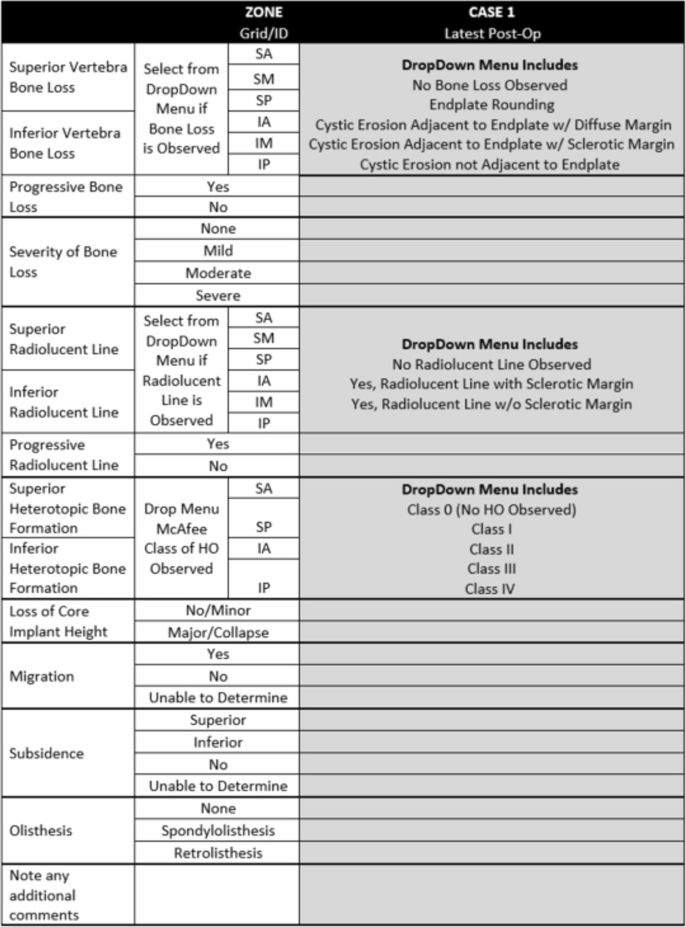
Case report form used to collect data

Protocol used for assessment of bone loss from radiographs

Gathering the data

The case series for the present study was an assembly of serial radiographs from cTDR cases by the spine surgeon investigators. The study protocol was reviewed by an external IRB and found to be IRB exempt.

For the present study, the serial radiographs from 19 patients with 25 implants were assembled and assessed using the classification system. The case series was assembled based on historical cases from the 4 spine surgeon investigators, and because radiographic changes were the focus of the assessment, inclusion of cases was based on availability of serial radiographs. For a case to be included, radiographs from pre-operative, post-operative, and latest follow-up timepoints had to be available, along with clinical presentation information. The pre-operative radiograph was crucial for understanding existing bone condition/anomalies prior to implant-related bone changes, and utilizing cases from a variety of manufacturers and designs helped reduce bias and focus on bone changes. Specific implantation duration was not required. The cases included the following implant systems: Discover (n = 1 patient, DePuy Spine), ProDisc-C (n = 2; Centinel Spine), Simplify (n = 2; NuVasive), M6-C (n = 5; Orthofix), Prestige LP (n = 2; Medtronic), Mobi-C (n = 9; ZimVie), and PCM (n = 4, NuVasive). There were 14 single-level patients, 4 two-level patients, and 1 three-level patient included as part of the study.

To simulate clinical situation as closely as possible, in evaluating case series, panel members considered patient reported symptoms throughout the course of their treatment and serial radiographs typically including index surgery, one-, two-, and five-years post-op. The 6 investigators were provided de-identified serial radiographs and clinical information for each case in the series. The clinical symptoms were used by the investigators to consider potential issues that might be observed in the radiographs, such as common bone loss scenarios, implant performance, potential bony abnormalities, or unique radiographic findings. This information was captured in the notes section of the data collection form (Fig. 4). Independently, each investigator reviewed each case according to the protocol, and provided observations using the data collection form. The data was then pooled, and statistical analyses conducted.

Statistical methods

The concordance between investigators was found by multiple pairwise comparison of investigator assessments. The maximum number of pairwise comparisons was 375. Concordance was determined by the number of paired observations, as compared with the total number of possible paired comparisons among investigators. Thus, if all of the paired comparisons in each of the region were consistent, that would result in 100% concordance or agreement (375 matching assessments out of a maximum 375 total possible assessments).

A random effects model was hypothesized as the data generating mechanism in order to evaluate the uncertainty in the estimates of overall agreement for each measurement. The model assumed that the 6 raters and 25 subjects were selected at random from populations of raters and subjects. A bootstrapping approach [31] was used to determine empirical sampling distributions for overall agreement. This was accomplished by creating 500 bootstrap samples by sampling 6 raters from the set of available raters with replacement and sampling 25 subjects from the set of available subjects with replacement; and then determining overall agreement as usual for each sample. The lower and upper bounds of the 95% confidence intervals were determined non-parametrically as the 2.5th and 97.5th percentile values. Agreement values smaller than lower bounds of the confidence intervals may be statistically ruled out. Overall agreement may be more interpretable in many cases than Kappa or Krippendorff’s Alpha values, which are very similar, are chance adjusted agreement rates but depend highly on prevalence of individual findings and marginal distributions (Fig. 5).

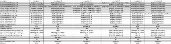
Example of case assessment data from six investigators