1 Introduction
Concrete creep is defined as the time-dependent deformation of a concrete specimen under sustained load. Its magnitude is closely related to the stress applied, time, cement type, mix proportion of concrete, and environmental conditions (ACI Committee 209, 2005). In practice, concrete creep can lead to additional displacements, stress redistribution, and even cracking in concrete structures during their service life (Hubert Rüsch and Hilsdorf, 1983; Bažant et al., 1997). As a result, a prestress loss is often observed in many large-scale prestressed concrete structures, such as long-span bridges and nuclear containments, which could significantly affect their safety and durability.
Under low stress, concrete can be considered an aging viscoelastic material, with concrete creep following the Boltzmann superposition principle. Thus, its strain rate can be expressed as (Bažant and Jirásek, 2018)
where is the age of concrete, is the time when the load is applied, is the first derivative of the compliance function with respect to , is the instantaneous elastic modulus, and and are the strain and stress rates, respectively. Equation (1) can be solved by the finite difference method. However, this method has some limitations. First, the entire stress history is required to obtain the strain increment at the current time step. As a result, in the process of solving creep by the finite element method, the entire stress history needs to be stored for the integration points of each element. For a large-scale problem with many time steps, the evaluation of these history variables is quite time-consuming. Second, the effects of some variable factors, such as temperature, humidity, and concrete cracks, cannot be considered.
It should be noted that the calculation method of comes from different creep models, reflecting the ratio of strain value to stress of the material at time (loaded at ), which is usually related to conditions such as material mix ratio, specimen shape, and environmental factors.
To overcome the difficulties of the finite difference method, Eq. (1) can be transformed into a differential rate-type equation, and an efficient exponential algorithm can be employed to calculate the concrete creep which exhibits a quadratic convergence rate and is unconditionally stable. Zienkiewicz et al. (1968) first applied this method to nonaging viscoelastic materials, and Bažant extended it to aging viscoelastic materials. This method can effectively improve computational efficiency with fixed internal variables. When using the efficient exponential algorithm, it is crucial to select a proper rheological model, such as the Kelvin chain model, to describe the viscoelastic behavior of the material. From a mathematical point of view, the creep compliance function of such a viscoelastic material can be approximated by the Dirichlet series. This can be achieved by curve fitting—the so-called retardation spectrum method.
The curve fitting method is usually based on the least squares method to obtain the coefficients of the Dirichlet series from test data. However, this method lacks actual physical meanings and does not follow the second law of thermodynamics, which sometimes leads to negative coefficients when the test data is not statistically ideal (Schapery, 1962). Many efforts have been made to solve the issue (Baumgaertel and Winter 1989; Elster and Honerkamp, 1991; Kaschta and Schwarzl, 1994; Mead, 1994; Emri and Tschoegl, 1995; Ramkumar et al., 1997; Park and Kim, 2001). Furthermore, for aging viscoelastic materials such as concrete, the coefficients of the Dirichlet series are time-dependent, and the curve fitting method becomes inefficient as the computational process needs additional optimization techniques.
With the continuous retardation spectrum method, the coefficients of the Dirichlet series can be determined by discretizing the continuous retardation spectrum, avoiding the issues encountered in the curve fitting method. Bažant and Xi (1995) studied the continuous retardation spectrum for concrete solidification theory and used the Post–Widder method to approximate the spectrum. In practice, however, a high-order Post–Widder formula is often needed to meet the precision requirement, which significantly increases the analytical complexity. Fortunately, Jirásek and Havlásek (2014) solved this issue using a low-order Post–Widder formula with time adjustment factors of retardation times. A high convergence speed and good accuracy are demonstrated for various concrete creep models. However, the method is heuristically based on empirical analyses, and the determination of time adjustment factors is highly dependent on personal experience and numerical experiments for different creep models.
The purpose of this paper is to develop an improved approach for efficiently approximating the continuous retardation spectra of various concrete creep models. The continuous retardation spectrum is first introduced, then the process of calculating the continuous retardation spectrum by the Post–Widder method and its corresponding shortcomings are analyzed, and an improved approach for solving the continuous retardation spectra based on the Weeks inverse Laplace transform method is proposed. By taking the CEB MC90 creep model as an example, the numerical solution of the continuous retardation spectra solved by the improved approach is analyzed. The proposed approach is then applied to the ACI 209R-92, JSCE, and GL2000 concrete creep models. Finally, the numerical results are compared with the other methods and some conclusions are drawn.
2 General solution for the continuous retardation spectrum
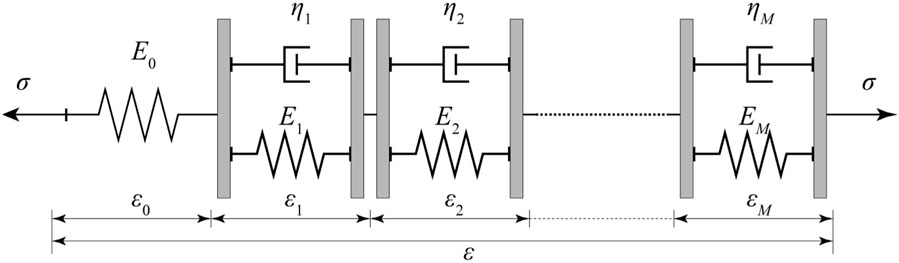
To describe viscoelastic materials, their constitutive properties can be represented by the Kelvin chain model. In the Kelvin chain model, the deformation of a material can be characterized by a number of Kelvin units and an additional spring unit assembled in series (Figure 1). Each Kelvin unit is composed of a spring and a dashpot assembled in parallel. All these units bear the same stress, and the total strain is equal to the sum of the deformations of each Kelvin unit and the spring unit.
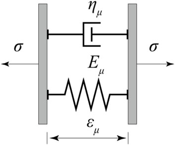
For the nonaging Kelvin unit shown in Figure 2, the total stress is equal to the sum of the elastic stress and the viscous stress.
where both the spring elastic modulus and the dashpot viscosity do not change with age.
For aging viscoelastic materials such as concrete, the aging Kelvin chain model is needed. For the aging Kelvin unit , the stress–strain relationship can be expressed in rate form as
where the modified age-dependent modulus is equal to
Since is equal to zero for creep tests, the boundary condition of is satisfied and the strain of the aging Kelvin unit can be obtained as
where is the retardation time of the Kelvin unit and is the time when the load is applied.
When the aging Kelvin chain model is subjected to a unit stress, the strains of all the Kelvin units () and the spring unit are superimposed; the compliance function is given by (Bažant, 1988)
which can be considered a finite Dirichlet series. In the practical application process, once the compliance function is constructed in the form of Eq. (7), the long-term creep value of materials can be numerically calculated by exponential algorithm. For a given time , when there are infinite number of Kelvin units in the chain and the retardation time distributes continuously, Eq. (7) can be converted into an integral form (Bažant and Xi, 1995):
where is the continuous retardation spectrum. For a specific creep model, once the continuous retardation spectrum is given, the direct discrete method can be used to construct the compliance function in the form of finite Dirichlet series. For convenience sake, the compliance function is rewritten as
where is the loading duration, and is defined as
By using the inverse Laplace transform method, Tschoegl (Nicholas, 1989) approximated from the Post–Widder method as
where is the th order derivative of . When , converges to the exact solution:
In this method, a sufficiently smooth function and a higher order are required for an acceptable approximation of the continuous retardation spectrum. This method is straightforward and efficient for some problems with simple compliance functions. In practice, however, the computation of the high-order derivatives is usually quite complicated, and the process of solving them will become complicated. To improve this method, Jirásek and Havlásek (2014) analyzed the difference between the low-order Post–Widder method and the exact solution and proposed an approach for adjusting the retardation time by multiplying correction factor to improve the accuracy of calculating continuous retardation spectrum. Thus, the continuous retardation spectrum is defined as
When the correction factor is applied, the accuracy of the numerical solution of the compliance function is effectively improved, and the approximation order is well controlled within low ranges. In this method, however, the value of the correction factor is determined empirically and is different for different creep models.
In Section 3, in view of the shortcomings of the Post–Widder method, an improved method for solving continuous retardation spectra based on the Weeks inverse Laplace transform is proposed. Here, Eq. (10) is processed in advance.
The differentiation of Eq. (10) with respect to yields
By setting , we have
It can be seen from Eq. (15) that is the Laplace transform of . Therefore, once the inverse Laplace transform of is determined, can be obtained.
3 Weeks method for the continuous retardation spectrum
In the method by Weeks (1966), the Laguerre polynomials are used to numerically calculate the inverse Laplace transform. The main advantage is that an explicit solution can be obtained. In applying this method, the following two conditions should be fulfilled: the Laplace space function is a smooth function with bounded exponential growth, and it can be expressed as a Laguerre series. The above two conditions are fulfilled for commonly used creep models, including the CEB MC90, ACI 209R-92, JSCE, and GL2000 models.
For Laplace space function , the analytical expression of the time-domain function can be obtained by the Weeks method as
In Eq. (16), and are two parameters that fulfill the conditions of and , where is the Laplace convergence abscissa. contains the information of the Laplace space function. It could be a scalar, vector, or matrix but does not change with time. With the Maclaurin series, the analytical expression of is given by
where is the radius of convergence of the Maclaurin series.
in Eq. (16) is the Laguerre polynomial of degree defined as
For practical numerical calculation, Eq. (16) can approximately be expressed as
where is an integer. The exact solution of can be obtained as approaches infinity
By using the Bromwich integral and the fast Fourier transform, an approximate expression of in Eq. (17) can be obtained as
where .
In the Laplace transform formula of Eq. (15), the Laplace space function is , the complex variable is , the time-domain function is , and the time-domain variable is . From Eq. (19), can be obtained through the inverse Laplace transform as
Substitution of into Eq. (22) leads to
In applying the Weeks method, it is obvious that the truncation error can be reduced by using a larger value of . In addition, a proper choice of and can lead to a higher convergence speed. Therefore, it is very important to choose the values of and reasonably. For Eq. (19), according to the method provided by Weeks (1966), when solving in the range of , the value can be simply determined as
For Eq. (23), let , and, considering that for all creep models , then and can be taken as
Equation (27) is simple and suitable for all creep models and can directly improve the computational accuracy by increasing , which is recommended to take a value between 10 and 50. In order to fully improve the computational efficiency, is taken as 10 in this paper, and, to further determine the values of and for different models, the analysis process is shown as follows.
To determine the parameters and , Weideman (1999) proposed a method by minimizing the theoretical error
where is the machine round-off error.
Further analysis according to the method of Weideman (Weeks, 1966), taking the CEB MC90 creep model (CEB-FIP, 1993) as an example, the compliance function is
where is the average elastic modulus of concrete at 28 days, is the correction factor related to the loading time , is the nominal creep coefficient related to the material strength, loading time, and the relative humidity of the environment, and the creep development coefficient is equal to
with being a coefficient related to the volume/surface ratio, the relative humidity, and the material strength, generally ranging from 250 to 1,500. By setting , the first-order derivative of is given by
When , , and are given, the error as a function of and can be obtained by substituting Eqs (24) and (31) into Eq. (28). should be selected by considering computational accuracy and efficiency. When a larger is used, the choice of and is more flexible.
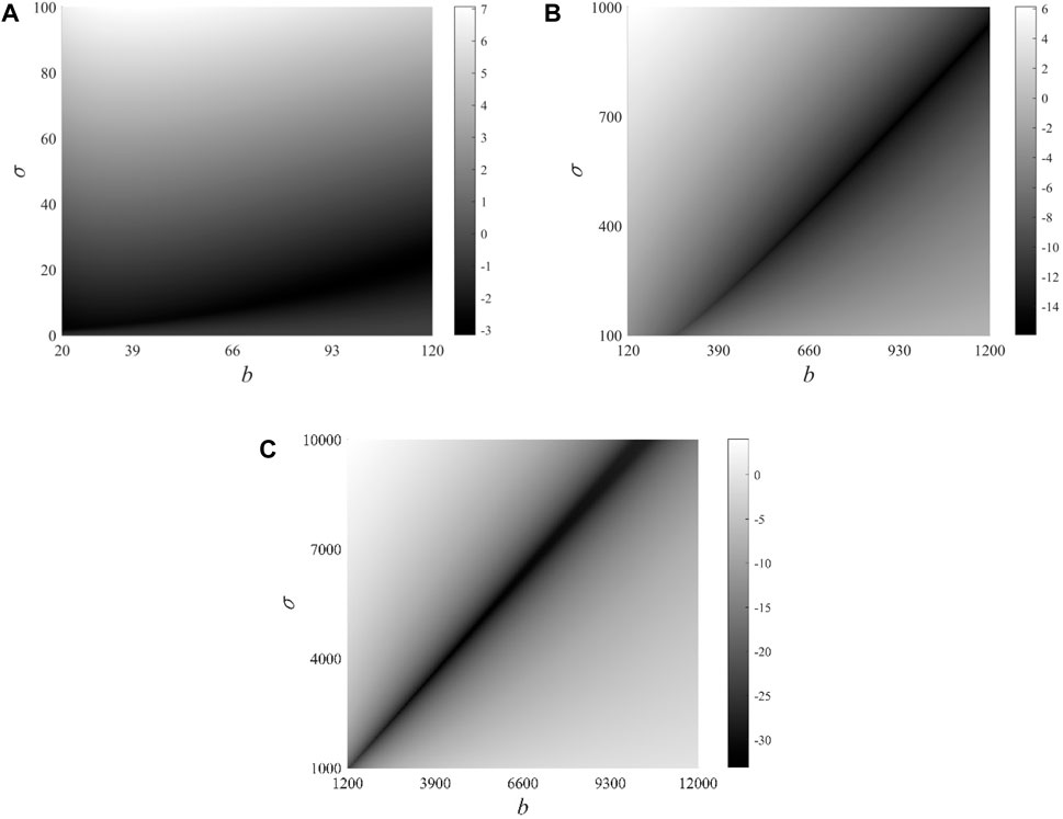
By setting and , is obtained as a function of and for different retardation times (Figure 3). The figure shows that the error can be significantly reduced by a proper choice of the two parameters. In some zones where and follow a certain relationship, the error is kept within relatively low levels as the dark part shown in Figure 3.
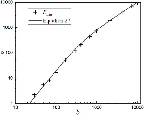
Combine the three graphs in Figure 3 and represent the horizontal and vertical coordinates in exponential growth. Select several points with the smallest error within different parameter ranges and use a few crosses to represent them, forming Figure 4.
If the relationship between and can be determined under the condition of minimum error , the method of parameter selection can be further determined. It was found that the relationship is related to the poles and branch points of the Laplace function (Weideman, 1999). If and are two farthest points to the origin of the Laplace function on the complex plane, we have
Equation (31) has two branch points: and . By using Eq. (32), the relationship between and for the CEB MC90 model can be obtained as
By taking , Eq. (33) is plotted as the solid line shown in Figure 4. It is apparent from Figure 4 that the numerical results from error minimization are very close to Eq. (33) for the CEB MC90 model. Therefore, for the CEB MC90 creep model, Eq. (33) can be determined as the relationship between and .
As seen from Eq. (23), the relationship between (or ) and is also required to perform the inverse Laplace transform and will be determined empirically through error analysis. Thus, a reference solution is obtained by a combination of the Durbin inverse Laplace transformation (Durbin, 1974) and an adaptive numerical integration. It should be pointed out that, although the reference solution has higher accuracy, it is very time-consuming and needs to be calculated by long-term iterative calculation and is thus not suitable for practical applications. The relative error is defined as
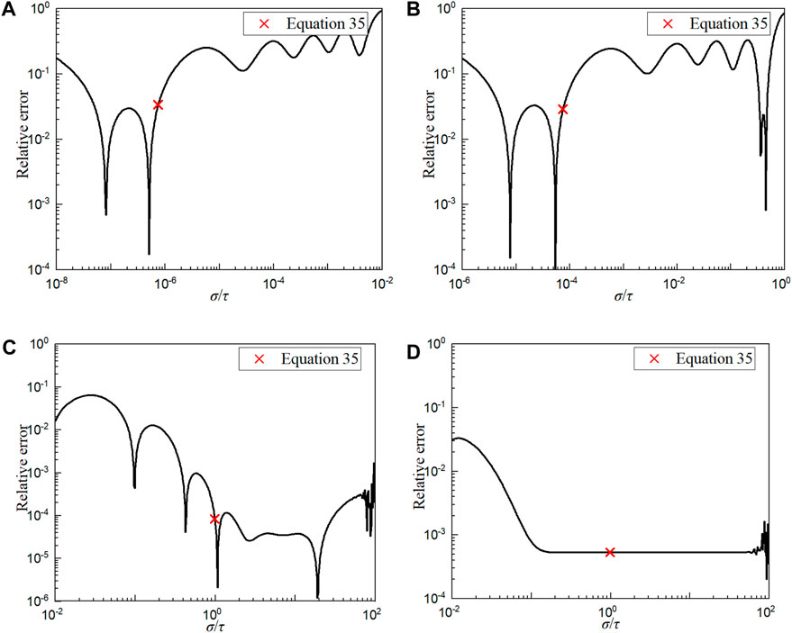
When , , under the premise of using Eq. (33) for parameter values, the relative errors of the Weeks inverse Laplace transform for are shown in Figure 5.
Figure 5 shows that, when is smaller than 1, the relative error exhibits larger changes from 10−4 to 1 (Figures 5A,B). When is larger than 100, the relative error is smaller than 10−1 and has a downward tendency as increases (Figures 5C,D).
Based on the numerical results in Figure 5, an empirical value of for the CEB MC90 model is suggested as follows:
For different values of , the relative error calculated from Eq. (35) is also obtained as the red cross shown in Figure 5. It is seen from Figure 5 that, when using Eq. (35), the relative error is smaller than 10−1. Particularly when is equal to 100 or 1,000, the relative error is smaller than 10−3. Therefore, computational accuracy is guaranteed.
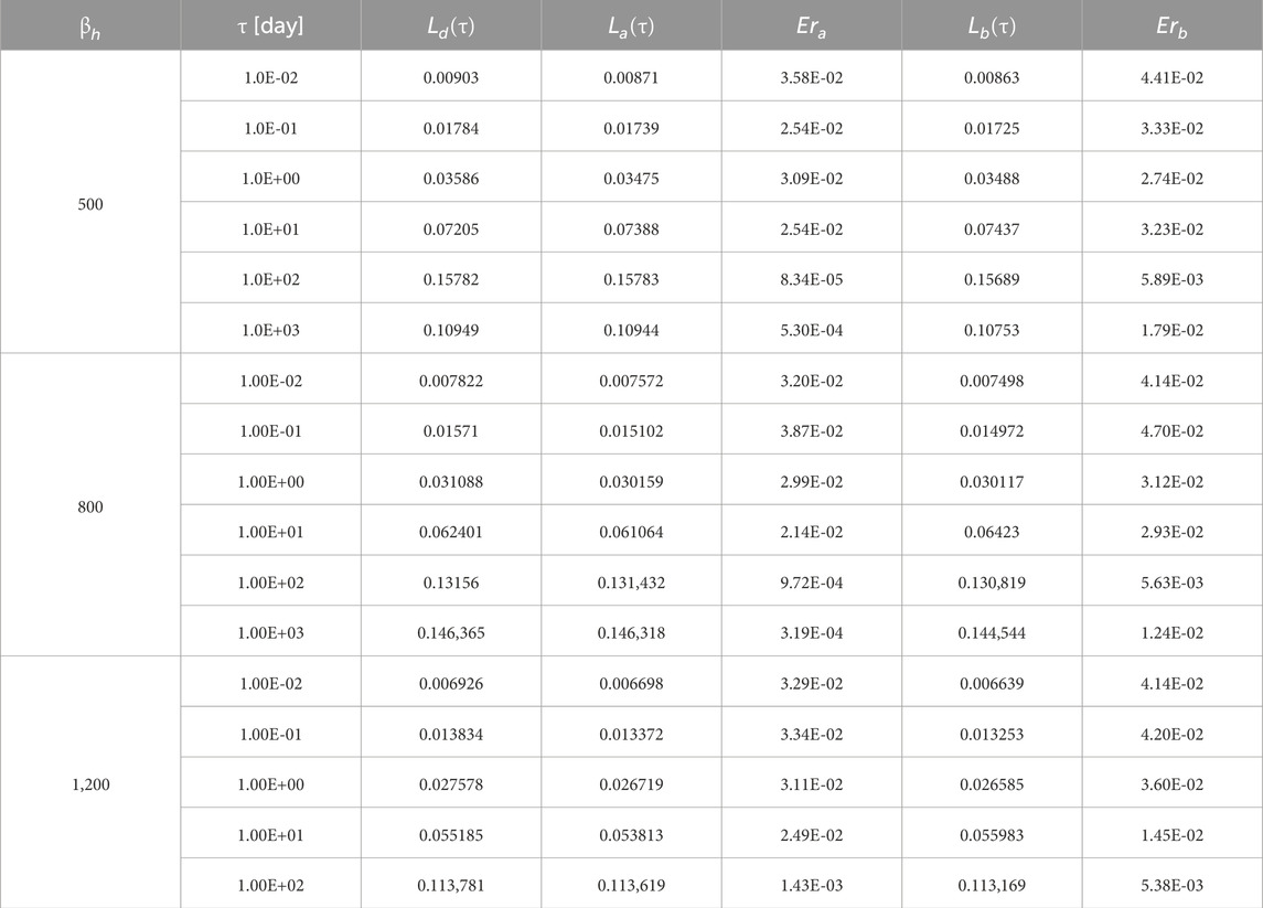
For and different values of , the continuous retardation spectra obtained from different methods are compared in Table 1, where is calculated from Eqs (33) and (35) while is calculated from Eq. (27), and are the relative errors between the calculated results obtained by the two calculation methods and the reference solution , respectively. It is seen from Table 1 that, compared with the Weeks parameter value method—Eq. (27)—the relative errors of the continuous retardation spectra given by Eqs (33) and (35) are smaller in most cases, and the computational accuracy is obviously improved. For the Weeks method, however, the computational accuracy can also be improved by increasing the value of .
4 Application of the Weeks method to different creep models
In this section, the Weeks method is applied to the CEB MC90, ACI 209R-92, JSCE, and GL2000 creep models. is calculated and analyzed based on the aging Kelvin chain and different methods for the continuous retardation spectrum. is used in all cases. The results obtained by a combination of the Durbin inverse Laplace transformation (Durbin, 1974) and an adaptive numerical integration are used as a reference solution.
4.1 CEB MC90 model
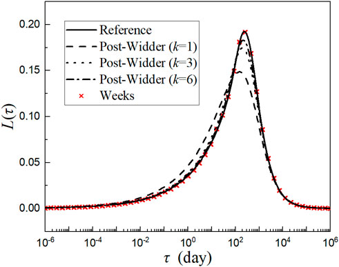
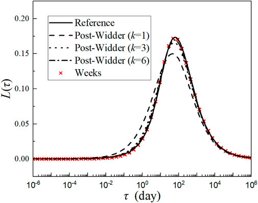
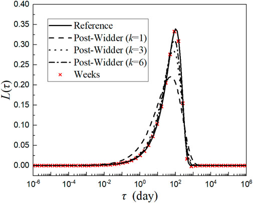
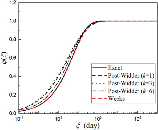
As discussed in the previous section, the continuous retardation spectrum of the CEB MC90 model can be obtained by the Weeks method. When , the continuous retardation spectra calculated by the Weeks method, the Post–Widder method with different orders, and the reference solution are shown in Figure 6.
Once is known, can be obtained from Eq. (10). However, the integral involved should be approximated by the Dirichlet series for an aging material. Therefore, the discrete retardation times are selected based on accuracy and efficiency. If is assumed to be a geometric series with an initial value of and a base of 10, that is,
then Eq. (10) is changed to
When , is close to unity, and the first term in Eq. (37) can be assumed to be , which is not affected by the duration . When , is close to zero, and the third term in Eq. (37) tends to be zero. Thus, Eq. (37) reduces to
The integral in Eq. (38) can be approximated by the two-point Gaussian quadrature rule:
The following definitions are used:
Equation (39) then becomes
If is set to be , of the aging Kelvin chain model is changed to
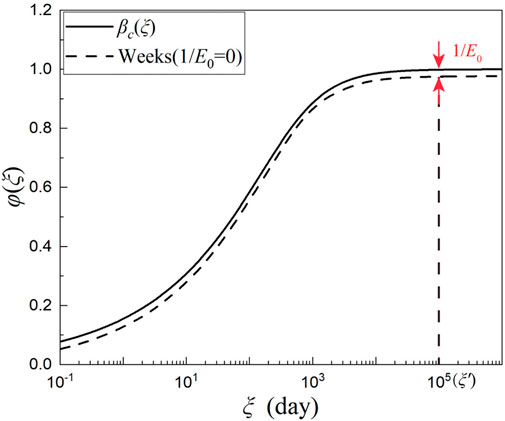
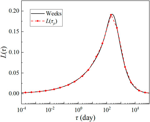
Equation (42) is consistent with the form of Eq. (7), where the number of Kelvin units is set to . can be obtained by numerical integration algorithms (Jirásek and Havlásek, 2014), but this will cause some errors. In this paper, in order to reduce the effect of numerical integration at low retardation times, is solved by subtracting the difference between the numerical solution and the exact solution of , which is in Eq. (30) for the CEB MC90 model:
where is the loading duration when reaches the maximum value ( for the CEB MC90 model). The analysis process is shown in Figure 7.
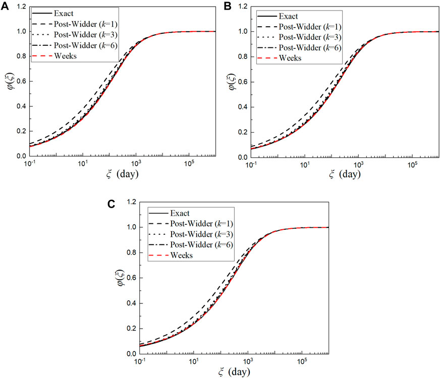
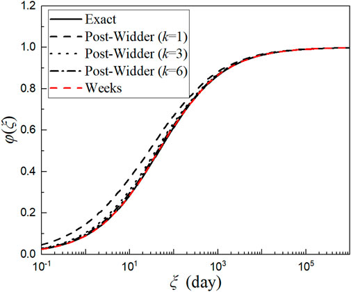
By taking as 500, 800, and 1,200, the values of are obtained by the Weeks and Post–Widder methods with different orders (Figure 8).
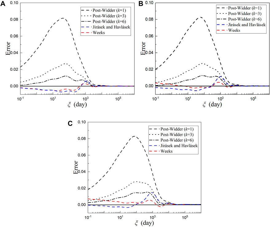
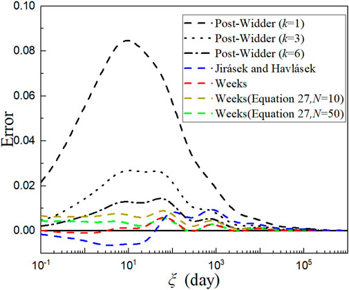
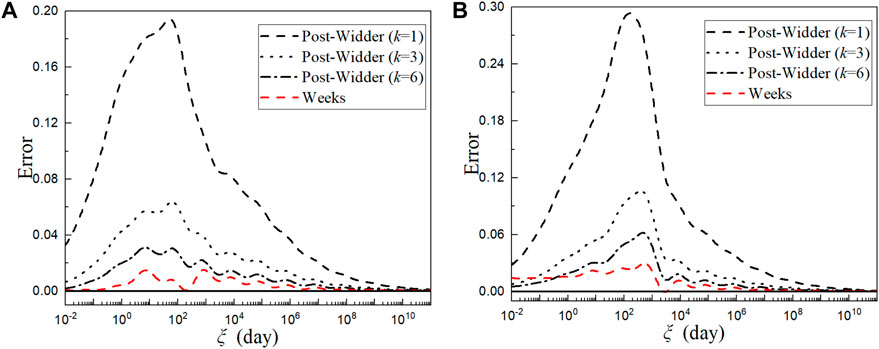
The error is defined as for the CEB MC90 model. Thus, the errors of different methods are shown in Figure 9. At the same time, the errors obtained from the method of Jirásek and Havlásek (2014) are also compared in Figure 9.
Equation (42) shows that is related to . For the two-point Gaussian quadrature rule, corresponding to different is able to describe the retardation spectrum curve as accurately as possible. If at two adjacent points are connected by line segments, the approximation of to the retardation spectrum curve can be observed more intuitively. As shown in Figure 10, the retardation spectrum curve can be described well when takes values from Eq. (40).
In Eq. (42), the number of Kelvin units is taken as 20. If higher computational accuracy is required, the number of Kelvin units can be increased: ). Thus, Eq. (42) becomes
where
It should be noted that, for most concrete creep models (CEB MC90, ACI 209R-92, and GL2000), the retardation spectra are relatively smooth, and taking in Eq. (45) usually satisfies the precision requirement. However, if the retardation spectrum changes sharply in terms of retardation time, it is necessary to increase the value of , which will be discussed in Section 4.3.
4.2 ACI 209R-92 model
The creep compliance function of the ACI 209R-92 model (ACI committee 209, 2008) is
where is defined as
In Eq. (50), is the ultimate creep coefficient related to the curing conditions, slump, and ambient humidity of concrete structures and and are two parameters—usually taken as 0.6 and 10 according to the recommendations in ACI 209R-92, respectively.
To simplify the analysis process, is defined as
Derivation of Eq. (51) with respect to gives
Since Eq. (52) has a branch point of , Eq. (32) cannot be directly used. For the ACI 209R-92 model, when , the computational accuracy of the creep compliance function obtained from Eq. (27) is not very satisfactory (Figure 13). With reference to the analysis of the CEB MC90 model, Eq. (28) is used to calculate and analyze the relationship between and . Thus is given by
When , the empirical expression of is expressed as
The continuous retardation spectra calculated by the Weeks method and the Post–Widder method with different orders are shown in Figure 11.
From Eq. (42), the values of of the ACI 209R-92 model for different durations are obtained as shown in Figure 12; the errors are shown in Figure 13. For comparison, the errors of calculated from Eq. (27) are also shown in Figure 13 for and . Figure 13 shows that, when Eq. (53) and (54) are adopted, the computational accuracy is obviously improved under the same value.
4.3 JSCE model
The creep compliance function of the JSCE model (Uomoto et al., 2008) is defined as
where is the ultimate creep strain under unit stress and related to the ambient relative humidity, temperature, and the volume/surface ratio. is defined as
Derivation of with respect to gives
Since Eq. (57) has only a branch point , Eq. (32) cannot be directly used to evaluate the values of and . Instead, Eq. (27) is adopted to determine the values of the two parameters. For , the continuous spectra calculated by the Weeks and Post–Widder methods with different orders are shown in Figure 14.
It is seen from Figure 14 that, compared with the CEB MC90 and ACI 209R-92 models, the continuous retardation spectra calculated by the Weeks method are steeper at the peak. The continuous retardation spectra of the CEB and ACI models show significant changes in the range from to , while that of the JSCE model mainly shows changes in the range from to . If is set in Eq. (45), cannot effectively describe the retardation spectrum curve. As shown in Figure 15A, the curve around is not well reproduced. Therefore, it is necessary to increase the value of . By setting the number of Kelvin units to — in Eq. (45)—it is seen from Figure 15B that the computational accuracy is greatly improved. Therefore, for the JSCE model, it is necessary to adopt this retardation time value method. The numerical results and the errors for different methods are shown in Figures 16, 17, respectively.
4.4 GL2000 model
The creep compliance function of the GL2000 model (Gardner and Lockman, 2002) is defined as
where is the elastic modulus at loading time and is the creep coefficient at 28 days. The expression of is
In Eq. (59), is the correction term for the drying effect before loading, is the relative humidity, and is the volume/surface ratio of specimens. To simplify the calculation, is expressed as
If and are defined as
the derivation of with respect to yields
Because the function form of is similar to Eq. (30), and the function form of is similar to Eq. (51), the parameter value forms of the CEB MC90 and ACI 209R-92 models can be referred to respectively. For , the values of and recommended for and are
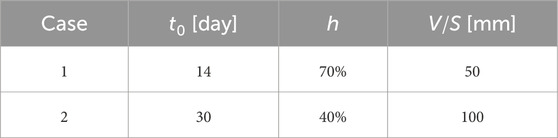
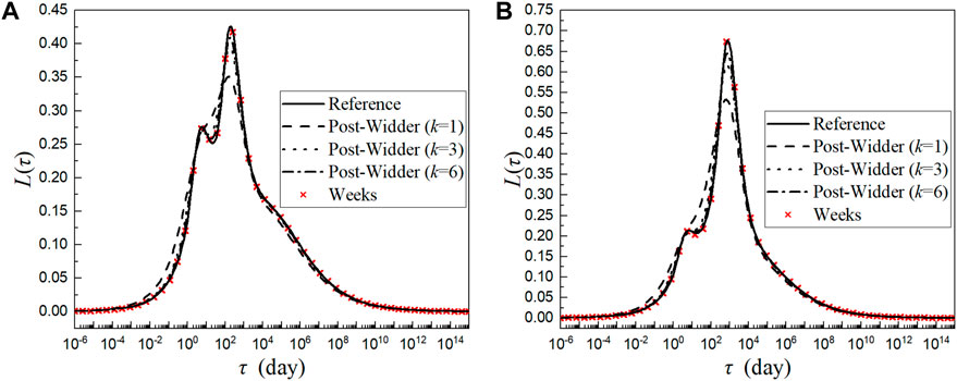
Two cases are considered, and the parameters are listed in Table 2. The continuous retardation spectra calculated by the Weeks and Post–Widder methods for different orders are shown in Figure 18.
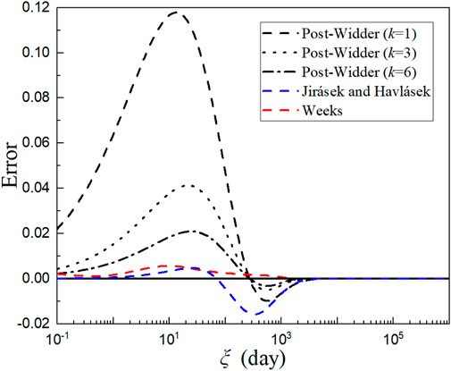
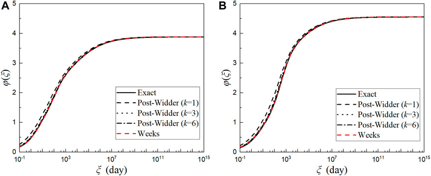
It is apparent from Figure 18 that the continuous retardation spectra begin to grow significantly from and decrease gradually at a long retardation time. Therefore, more Kelvin units are needed to cover the range of the continuous retardation spectra. Consequently, is set to , the maximum value of in Eq. (36) is taken as 18, for this model, and the number of Kelvin units in Eq. (42) changes from 20 to 36. The values of of the GL2000 model for different duration are obtained as per Figure 19, and the errors are shown in Figure 20. Since the GL2000 model was not discussed by Jirásek and Havlásek (2014), the error obtained from their method is not compared in Figure 20.
4.5 Discussion
For all the concrete creep models discussed in this section, the proposed approach based on the Weeks method improves the computational accuracy and efficiency of the continuous retardation spectra and the creep compliance. It should be noted that, for the case of long duration, the errors of decrease with the increase of and approach zero. There are two main reasons for this phenomenon. First, the creep compliances used have negligible variation for a long duration and have a clear upper limit. Thus, the approximation through the Dirichlet series will maintain the same characteristics as long as the retardation time range selected is wide enough. Second, by calculating based on the most accurate compliance value—Eq. (43)—the effect of numerical integration for a short duration on the final results is reduced.
For the creep models considered, when , the absolute error of given by the improved approach (using the Weeks method) is smallest and maintains a lower level (usually smaller than 0.01). For the ACI 209R-92 and JSCE models, the results from the proposed approach achieve higher accuracy than the Post–Widder method. When calculated by the improved approach, of the ACI 209R-92 model is closest to the reference solution, while of the JSCE model exhibits the most significant improvement on the Post–Widder method.
The errors of obtained from the improved approach and the Jirásek–Havlásek method are both controlled at a relatively low level. For the CEB MC90 model, the results obtained from Jirásek–Havlásek are more accurate for low retardation times, while those obtained from Weeks are more accurate for high retardation times. As shown in Figure 9, the errors corresponding to the Weeks method are smaller compared to the Jirásek–Havlásek method when . For the ACI 209R-9 and JSCE models, the results obtained from Weeks are more accurate and the errors of are smaller.
For the other creep models which are not discussed in this paper, the proposed approach is still applicable when they fulfill the requirement of the Weeks inverse transform. In general, a large value of can be used to achieve the required computational accuracy and a proper choice of and can significantly improve computational efficiency. In general, Eq. (27) can be used to determine the parameters, and is recommended. The larger the value of , the more accurate the calculation results, but computational efficiency will be reduced. If has two or more poles and branch points, Eq. (32) can also be used to determine the parameters, and precision requirements are usually satisfied when .
5 Comparison with experimental results
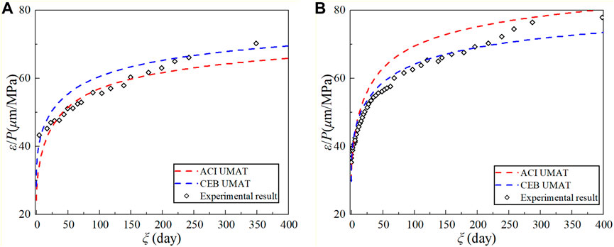
To further verify the validity of the improved approach, the finite element method is used to compute the long-term creep of concrete by combining the retardation spectrum obtained by the Weeks method with the second-order exponential algorithm (Bažant and Jirásek, 2018). For this purpose, two sets of experimental data, OPC and SF10, were selected from Mazloom et al. (2004). They had different mix proportions, and a pressure of 10 MPa was applied on the OPC and SF10 cylinders on the 28th and 7th days, respectively. Two UMAT user subroutines for material behavior—ACI UMAT and CEB UMAT—of the commercial finite element software ABAQUS were coded. The concrete strain was calculated using the CEB MC90 and ACI 209R-92 creep models. The results are shown in Figure 21, which shows that the finite element results are in good agreement with the experimental results. For the OPC group, the ACI 209R-92 model has higher accuracy, while, for the SF10 group, the CEB MC90 has higher accuracy.
It is noted that one of the purposes of this paper is to ensure that the numerical results agree well with the corresponding expressions of . As a result, the accuracy of the final numerical results is mainly dependent on whether the analytical expression of given by design codes is close to the practical situation. Therefore, before the concrete creep is calculated, it is necessary to select a reasonable model according to the practical situation, including the mix proportion, the component shape, loading, and environmental conditions, to ensure the computational accuracy of the numerical results. It should also be noted that, since this paper is mainly concerned with improving on the continuous retardation method, finding a viable, stable strategy to identify the optimal dimension of the approximation in the presence of an error (uncertainty) on data is not addressed. This limitation is expected to be removed in our future work.
6 Conclusion
Based on the Weeks method, an efficient approximation approach has been developed for the continuous retardation spectra of aging viscoelastic materials. Compared with the existing methods, the approach has several advantages.
(1) It can calculate the continuous retardation spectrum more accurately by only using the first-order derivative of the creep compliance function. The difficulty of calculating the high-order derivatives in the Post–Widder method is avoided.
(2) Unlike the method proposed by Jirásek and Havlásek (2014), in which the correction factor is empirically determined for each concrete creep model at a given derivative order, the proposed approach is based on a solid theoretical foundation and can be conveniently applied to various concrete creep models.
(3) Better computational accuracy can be achieved for a long loading duration. As illustrated by different concrete creep models, the error of the creep compliance function obtained by the proposed approach is controlled within 0.02 for a loading duration of . Therefore, the approach is applicable to long-term creep analyses of aging viscoelastic materials, such as concrete.
It should be noted that the proposed approach is only applicable to concrete creep models when the first-order derivative of the compliance function fulfills the requirement of the Weeks method. For concrete creep models with logarithmic compliance functions, such as the fib model (CEB-FIP, 2010), the inversion formula of the Laplace transform has an analytical solution and does not require the Weeks method for the continuous retardation spectrum. In this research, to achieve high computational efficiency and accuracy, the values of and for the CEB MC90, ACI 209R-92, and GL2000 models are determined empirically for . As for the JSCE model, a good precision requirement can be achieved when the parameters are taken directly through Eq. (27) for . If the proposed approach is applied to other creep models, the parameters can be determined by referring to the analytical process of this paper or directly by increasing the value of to meet the precision requirements.
Data availability statement
The raw data supporting the conclusion of this article will be made available by the authors, without undue reservation.
Author contributions
XZ: Conceptualization, Methodology, Writing–review and editing. LB: Formal Analysis, Validation, Writing–original draft. HR: Data curation, Software, Writing–original draft. XF: Funding acquisition, Project administration, Supervision, Writing–original draft. JZ: Funding acquisition, Resources, Writing–review and editing. YG: Investigation, Visualization, Writing–original draft.
Funding
The author(s) declare financial support was received for the research, authorship, and/or publication of this article. This research was funded by the National Science Foundation for Excellent Young Scholars (Grant No. 52222808), the Zhejiang Provincial Natural Science Foundation (Grant No. LY20E080027), and the National Natural Science Foundation of the People’s Republic of China (Grant Nos 52008413, 52078509, 52178255, and 52278279).
Conflict of interest
Authors HR, XF, and YG were employed by Metallurgical Group Corporation of China.
The remaining authors declare that the research was conducted in the absence of any commercial or financial relationships that could be construed as a potential conflict of interest.
The handling editor J-GD declared a past co-authorship with the author JZ.
Publisher’s note
All claims expressed in this article are solely those of the authors and do not necessarily represent those of their affiliated organizations, or those of the publisher, the editors, and the reviewers. Any product that may be evaluated in this article, or claim that may be made by its manufacturer, is not guaranteed or endorsed by the publisher.
Supplementary material
The Supplementary Material for this article can be found online at: https://www.frontiersin.org/articles/10.3389/fmats.2024.1340883/full#supplementary-material
References
ACI Committee 209 (2005). Report on factors affecting shrinkage and creep of hardened concrete. Farmington Hills: American Concrete Institute.
Google Scholar
ACI Committee 209 (2008). Guide for modeling and calculating shrinkage and creep in hardened concrete. Farmington Hills: American Concrete Institute.
Google Scholar
Baumgaertel, M., and Winter, H. H. (1989). Determination of discrete relaxation and retardation time spectra from dynamic mechanical data. Rheol. Acta 28, 511–519. doi:10.1007/BF01332922
CrossRef Full Text | Google Scholar
Bažant, Z. P. (1988). Mathematical modeling of creep and shrinkage of concrete. New York: John Wiley and Sons.
Google Scholar
Bažant, Z. P., Hauggaard, A. B., Baweja, S., and Ulm, F. J. (1997). Microprestress-solidification theory for concrete creep. I: aging and drying effects. J. Eng. Mech. 123, 1188–1194. doi:10.1061/(asce)0733-9399(1997)123:11(1188)(1997)123:11(1188)
CrossRef Full Text | Google Scholar
Bažant, Z. P., and Jirásek, M. (2018). Creep and hygrothermal effects in concrete structures. Netherland: Springer Dordrecht.
Google Scholar
Bažant, Z. P., and Xi, Y. (1995). Continuous retardation spectrum for solidification theory of concrete creep. J. Eng. Mech. 121, 281–288. doi:10.1061/(asce)0733-9399(1995)121:2(281)(1995)121:2(281)
CrossRef Full Text | Google Scholar
CEB-FIP (1993). Design of concrete structures, CEB-FIP model-code 1990. London: British Standard Institution.
Google Scholar
CEB-FIP (2010). Fib Model Code for concrete structures 2010. London: British Standard Institution.
Google Scholar
Durbin, F. (1974). Numerical inversion of laplace transforms: an efficient improvement to dubner and abate’s method. Comput. J. 17, 371–376. doi:10.1093/comjnl/17.4.371
CrossRef Full Text | Google Scholar
Elster, C., and Honerkamp, J. (1991). Modified maximum entropy method and its application to creep data. Macromolecules 24, 310–314. doi:10.1021/ma00001a047
CrossRef Full Text | Google Scholar
Emri, I., and Tschoegl, N. W. (1995). Determination of mechanical spectra from experimental responses. Int. J. Solids Struct. 32, 817–826. doi:10.1016/0020-7683(94)00162-P
CrossRef Full Text | Google Scholar
Gardner, N. J., and Lockman, M. J. (2002). Design provisions for drying shrinkage and creep of normal-strength concrete. ACI Mater. J. 98, 159–167. doi:10.14359/10199
CrossRef Full Text | Google Scholar
Hubert Rüsch, D. J., and Hilsdorf, H. K. (1983). Creep and shrinkage. New York: Springer.
Google Scholar
Jirásek, M., and Havlásek, P. (2014). Accurate approximations of concrete creep compliance functions based on continuous retardation spectra. Comput. Struct. 135, 155–168. doi:10.1016/j.compstruc.2014.01.024
CrossRef Full Text | Google Scholar
Kaschta, J., and Schwarzl, R. R. (1994). Calculation of discrete retardation spectra from creep data-Ⅰ. Method. Rheol. Acta 33, 517–529. doi:10.1007/BF00366336
CrossRef Full Text | Google Scholar
Mazloom, M., Ramezanianpour, A. A., and Brooks, J. J. (2004). Effect of silica fume on mechanical properties of high-strength concrete. Cem. Concr. Compos. 26, 347–357. doi:10.1016/s0958-9465(03)00017-9
CrossRef Full Text | Google Scholar
Mead, D. W. (1994). Numerical interconversion of linear viscoelastic material functions. J. Rheology 38, 1769–1795. doi:10.1122/1.550526
CrossRef Full Text | Google Scholar
Nicholas, W. T. (1989). The phenomenological theory of linear viscoelastic behavior. Heidelberg: Springer.
Google Scholar
Park, S. W., and Kim, Y. R. (2001). Fitting prony-series viscoelastic models with power-law presmoothing. J. Mater. Civ. Eng. 13, 26–32. doi:10.1061/(asce)0899-1561(2001)13:1(26)(2001)13:1(26)
CrossRef Full Text | Google Scholar
Ramkumar, D. H. S., Caruthers, J. M., Mavridis, H., and Shroff, R. (1997). Computation of the linear viscoelastic relaxation spectrum from experimental data. J. Appl. Polym. Sci. 64, 2177–2189. doi:10.1002/(SICI)1097-4628(19970613)64:11<2177::AID-APP14>3.0.CO;2-1
CrossRef Full Text | Google Scholar
Schapery, R. (1962). “A simple collocation method for fitting viscoelastic models to experimental data“, in: Graduate Aeronautical Laboratory. (California: California Institute of Technology).
Google Scholar
Uomoto, T., Ishibashi, T., Nobuta, Y., Satoh, T., Kawano, H., Takewaka, K., et al. (2008). Standard specifications for concrete structures-2007 by Japan society of Civil engineers. Concr. J. 46, 3–14. doi:10.3151/coj1975.46.7_3
CrossRef Full Text | Google Scholar
Weeks, W. T. (1966). Numerical inversion of laplace transforms using Laguerre functions. J. ACM 13, 419–429. doi:10.1145/321341.321351
CrossRef Full Text | Google Scholar
Weideman, J. a.C. (1999). Algorithms for parameter selection in the weeks method for inverting the laplace transform. Siam J. Sci. Comput. 21, 111–128. doi:10.1137/s1064827596312432
CrossRef Full Text | Google Scholar
Zienkiewicz, O. C., Watson, M., and King, I. P. (1968). A numerical method of visco-elastic stress analysis. Int. J. Mech. Sci. 10, 807–827. doi:10.1016/0020-7403(68)90022-2
CrossRef Full Text | Google Scholar


Add Comment