Nodule segmentation
We observed a smooth decrease in the training loss with a fluctuated mean dice score in the validation loss due to the overfitting of the model. Therefore, we include a dropout rate of 20% during each epoch. Example cases of the segmentation results are shown in Fig. 3 for the LIDC dataset and the in-house dataset. We were able to see the similarity between the ground truth and the generated mask. We achieved an average dice score of 0.761 on the validation dataset after 50 epochs of training. The ADAM optimizer was used with the learning rate and dropout rate as 0.0001 and 0.2, respectively. Data augmentation, including random flips, intensity scaling, and intensity shifting, were used to improve model performance. The dice loss function was used as a metric to access the model performance and evaluate the testing dataset. The sliding window inference method which uses a rectangular or cube region of fixed dimension that “slides” across an image was applied to create binary classifications on whether or not each voxel belongs to a nodule. Although computationally expensive, this method determines if the window has an object that interests us. Accelerated methods such as cache IO and transform function featured by MONAI were also used to expedite the training process.
All experiments including preprocessing, developing, and evaluation of the model, were performed using Python version 3.6 and PyTorch 1.5 on NVIDIA GP102, GTX 1080 Ti.
3D AG-Net Pre-training on LIDC-IDRI
To ensure the effectiveness of the 3D AG-Net for the nodule malignancy classification task, we validated the classification model using the LIDC dataset, which has public benchmarks. The model was trained with an early stopping strategy with patience of 50 epochs based on the highest validation accuracy. The network used binary cross-entropy (BCE) loss for nodule malignancy classification. The input data is a 64 × 64 × 64 voxel CT nodule image, Adam optimizer with an initial learning rate set at 0.0002, batch size 128. All experiments were conducted on an Nvidia GTX 1080 Ti GPU with PyTorch library. We achieved 91.57%, 83.34%, 90.46%, and 0.95 for accuracy, sensitivity, precision, and AUC, respectively, with the S1 and S2 (benign) versus S4 and 5 (malignant), which is compatible with the state-of-the-art models’ performances (Additional file 1: Appendix SC). The result trained with the complete LIDC dataset, S1, S2, S3 (benign) versus S4 and S5 (malignant), also reported here as 85.11%, 77.78%, 88.54%, and 0.90 ± 0.04 for accuracy, sensitivity, specificity, and AUC, respectively (Table 2). Although the model trained with the complete LIDC dataset achieved lower metrics scores, it serves as a better initializer for the training of the in-house dataset since the complete dataset better reflects the real-world conditions. Therefore the model is more generalized for later applications.
3D AG-Net training on the in-house dataset
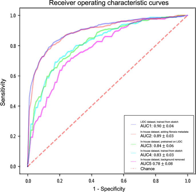
For models trained with the in-house dataset with tenfold cross-validation, the experiment results are summarized in Table 2 and Fig. 4. The performance of the 3D AG-Net without pretraining (trained from scratch) achieved 78.84 ± 5.88%, 62.00 ± 13.65%, 87.29 ± 5.98%, 0.83 ± 0.03 for accuracy, sensitivity, specificity, and AUC, respectively. The model with pretraining on LIDC dataset achieved results of 79.03 ± 2.97%, 65.46 ± 18.64%, 85.86 ± 6.29%, 0.84 ± 0.06 for accuracy, sensitivity, specificity, and AUC, respectively. When the background information was removed, it performed slightly worse in most of the metrics except for specificity, achieving 75.61 ± 7.02%, 50.00 ± 25.46%, 88.46 ± 7.88%, 0.78 ± 0.08 for accuracy, sensitivity, specificity, and AUC, respectively. When additional semantic fibrosis metadata was provided, the 3D AG-Net yielded the best AUC when comparing all other types of datasets. The result was 80.84 ± 3.31%, 74.67 ± 14.78%, 84.95 ± 5.43%, 0.89 ± 0.05 for accuracy, sensitivity, specificity, and AUC, respectively.
Receiver operating characteristic (ROC) curves and area under the curves (AUC) of experiments with different datasets and methods. The ROC curves demonstrated here are the averaged ROC based on the tenfold cross-validation. The averaged AUCs with one standard deviation are computed and listed in the legend area. The blue line, red line, green line, cyan line, magenta line, and the red dashed-line are indicating the nodule malignancy prediction results on the LIDC dataset, In-house dataset with metadata, In-house dataset (pretrained with LIDC), In-house dataset, and In-house dataset (background removed), respectively. Statistical differences were found in 1 LIDC dataset, trained from sketch v.s. In-house dataset, trained from sketch (p-value: 0.0319); 2 LIDC dataset, trained from sketch v.s. In-house dataset, background removed (p-value: 0.0001); 3 In-house dataset, adding fibrosis metadata v.s. In-house dataset, background removed (p-value: 0.0002)
We used 3D AG-Net without pretraining as the baseline to compare with the model pretrained on LIDC dataset (AUC increase 1.2%), the model trained with background removed (AUC decrease 6%, p-value < 0.01), and model trained with additional semantic fibrosis metadata (AUC increase 7.2%, p-value < 0.01). We found statistical differences (p-value < 0.01) in AUC between adding (model trained with additional semantic fibrosis metadata) and removing (model trained with nodule background removed) fibrosis information. When semantic fibrosis information is available to the network, the nodule malignancy classification accuracy increases 5.23%. Nodule volume doubling time (VDT) as the current clinical guideline to predict nodule malignancy is also included in the experiment for comparison. The VDT method achieved 62.63%, 56.52%, and 65.48% of accuracy, sensitivity, and specificity respectively. Note that CNN trained with nodule-only images still outperformed the VDT method.
The 3D AG-Net was also trained with the in-house dataset to predict lung fibrosis using the ground-truth fibrosis diagnosis provided by radiologists (fibrosis as 1, non-fibrosis as 0). The model achieved 73.01 ± 5.84%, 75.18 ± 13.32%, 70.83 ± 6.22%, and 0.75 ± 0.07 for accuracy, sensitivity, specificity, and AUC, respectively.
Visualization
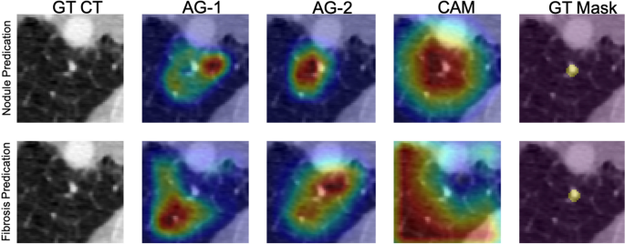
Figure 5 depicts network visualizations for nodule and fibrosis classification. Notably, distinct attention patterns emerge within the same case when different objectives, such as nodule or fibrosis classification, are employed.
Network attention gates (AGs) and class activation maps (CAMs) visualizations. An example is network visualization for nodule prediction (first row) and lung fibrosis prediction (second row) tasks. The first, second, third, and fourth columns indicate the ground-truth (GT) CT image, first attention gate (AG-1) at No. 11 layer depth, second attention gate (AG-2) at No. 14 layer depth, and the class activation map (CAM) at the final layer, respectively. The fifth column indicates the nodule ground-truth mask (GT Mask), which is not available when the model was trained. The case demonstrated here is a benign nodule in the non-fibrotic lung, where both nodule malignancy and fibrosis models made the correct inferences. From the AGs and CAMs, we can observe the nodule network focuses on nodule parenchyma and its surrounding tissues, while the fibrosis network focuses on other lung tissue with the nodule parenchyma excluded
For nodule classification, the network exhibits a similar attention pattern for true positive cases (Fig. 6a) and false positive cases (Fig. 6b). AG-1 surveys the nodule and the microenvironment, AG-2 removes the attention on the nodule and surveys the surrounding microenvironment, and CAM at the last layer shifts the attention back to the nodule parenchyma. For true negative cases (Fig. 6c) and false negative cases (Fig. 6d), another attention pattern is observed. The network attention starts with AG-1 the nodule and the microenvironment. Sequentially at the AG-2 layer, the network removes the attention from the majority of the nodule parenchyma with a focus on the microenvironment. At the final stage, the network completely removes the attention from the nodule.
Results of the 3D AG-Net on the in-house dataset. A true positive case (a), a false positive case (b), a true negative case (c), and a false negative case (d) were shown. In each case, it showed the center slice of the 64 × 64 × 64 volume, the slice with the AG-1 heatmap, the slice with the AG-2 heatmap, and the slice with CAM on top of it from left to right, respectively
In summary, the network conducts similar search patterns at AG-1 and AG-2 stages for all the cases, then if the network attention shifts back to the nodule at the final stage, the classification will be malignant, while the attention remains at the microenvironment, the classification will be benign. In Fig. 6., We demonstrate cases of four possibilities including true positive (a), false positive (b), true negative (c), and false negative (d). It also presents the attention-gated maps and CAM of each case from left to right, respectively. We found that false positive cases usually occurred with larger nodule sizes, especially when the nodule size exceeds our per-defined 64 × 64 × 64 ROI, therefore, there is limited nodule shape, boundary, and microenvironment information presented to the network. For false negative cases, nodules with less diffuse characteristics and more well-defined boundaries are more likely to be classified as benign by the network.
As for fibrosis classification, the network initially searches the surrounding soft tissue area close to the nodule and gradually enlarges the survey area in lung parenchyma to detect fibrotic tissues.


Add Comment