Data and data management
Data currently consists of the entire Danish population aged 45 or older on January 1, 2018, coupled with a 15-year look-back (2003–2017) in the Danish national registries, and these data are used in the analyses reported in the current article. We intend to update the data to include later years, before performing the analyses outlined in this protocol. Included individuals are observed for a period of 1 year from the index date, during which outcomes may occur. The 15-year look-back is used to collect information on personal characteristics and exposures, and we refer to these collectively as predictors. Other fracture prediction studies employ cohorts that are slightly younger (40 years and older [18,19,20]) or older [21,22,23]. Trémollieres and colleagues argue that a cutoff at 45 years allows for the inclusion of early menopausal women, who may be at increased risk of osteoporotic fracture [24]. The sample size is dictated by the study design and the data obtained from the Danish national registries. The original FREM study included a sample of 2,495,339 individuals [12].
Data sources largely coincide with those used for the original FREM tool [12], except that the present model also utilizes information on medicine redemptions and uses an updated data extraction from the registries. All data management and analyses are performed on a secure server at the Danish Health Data Authority.
Data sources
Data is extracted from a collection of Danish health registries. The Danish health registries cover all citizens of Denmark and offer long-term data on the entire population and may generally be characterized as having a high degree of validity and completeness [25]. Data from the following three national registries are used in this study:
-
The Danish Civil Registration System (CRS) includes all individuals residing in Denmark [26]. Upon birth or immigration, an individual is assigned a unique person identification number which may be used to identify the individual across registries [27]. The CRS is used to identify the study population and to determine age and sex.
-
The Danish National Patient Register (NPR) is an administrative register containing all inpatient, outpatient, and emergency department contacts from Danish hospitals, since 1977 (outpatient and emergency departments since 1995) for both public and private hospitals (private hospitals since 2003) [28]. Records contain information on clinical characteristics along with procedures and treatment, in particular the diagnosis (-es) associated to the contact. The NPR is used to identify the outcomes of interest along with predictors using ICD-10 (International Classification of Diseases 10th Revision)-coding.
-
The Danish National Prescription Registry (DNPR) contains individual-level data on all dispensed prescription pharmaceuticals sold in Danish community pharmacies [29]. Data comprises information on ATC (Anatomical Therapeutic Chemical Classification System)—codes, price reimbursement, etc., at the redemption level. The DNPR is used to define predictors.
Outcome definitions
Two outcomes will be considered, a major osteoporotic fracture (MOF) or a hip fracture (HF). The primary outcome is MOF, defined as fracture of hip, clinical vertebral, wrist, or humerus (given as a primary or secondary ICD-10 code in the NPR: S120, S121, S122, S220, S221, S320, T08, S422, S423, S720, S721, S722, S525, or S526) [12] (Table 1). The secondary outcome is HF, which is given as a primary or secondary ICD-10 code in the NPR (S720, S721, or S722) [12] in combination with a surgical code (KNFB, or one of its sub-codes, or KNFJ4x-9x) [30]. Both definitions of MOF and hip fractures will be evaluated in a forthcoming medical record review and will potentially be updated following the results of this review.
Diagnoses as predictors
Information is collected on all non-administrative level 3 ICD-10 codes. We record both the occurrence and date of each ICD-10 code. If more than one instance of the same diagnosis occurs in the look-back period, the first record is used. Note that previous experiences of an osteoporotic fracture thus enter as predictors through the ICD10 codes and that those with previous fractures are not excluded. The diagnosis exposure is defined as the time from the first diagnosis to the end of the look-back period.
Rare diagnoses are excluded based on the unsupervised review as described below.
Pharmacological exposures from redemptions
Redemptions (i.e., prescriptions filled) are perceived as relevant risk predictors in two ways. First, the redemption may act as a proxy for a diagnosis that is not recorded through the administrative health registers under consideration. This may occur since the NPR contains information on diagnoses from hospital contacts only and not from general practice consultations. Diagnosis registrations from general practice are difficult to retrieve for research purposes as they are not registered in a national database but in systems provided by privately owned software providers. However, data on redemptions of prescription drugs prescribed by general practitioners can be retrieved from the DNPR and redemptions may therefore act as proxies for diagnoses from general practice. Secondly, the redemption may signify exposure to a pharmaceutical with effects on fracture risk, which may influence the risk of outcome by e.g., affecting the individual’s bone density or by altering the risk of experiencing a serious fall. The second class of pharmaceuticals with effects on fracture risk are further subsets depending on their assumed type of effect. We record whether the ATC code was redeemed during the look-back period and further record a measure of the extent of exposure. The following pharmaceutical exposures are used:
-
1.
Medications associated with risk of developing osteoporosis: Defined by the ATC codes in Table 2 (taken from [31]). Exposure is coded as time (in days) from the earliest redemption in the look-back period and defined as zero if no redemption occurred.
-
2.
Fall-specific: Table 3 gives an overview of pharmaceuticals related to fall risk and the associated ATC codes. Their exposure is coded as 15 times 365.25 (i.e., the number of days in the lookback period) minus the number of days from the last redemption during the look-back period and is defined to be zero if no redemption occurred. Thus, a high exposure signifies a very recent redemption.
-
3.
Diagnosis proxies: ATC codes to be used as proxies for diagnoses are all non-osteoporosis-specific codes included on the therapeutic level of the ATC hierarchy (level 3), meant to reflect the same therapeutic areas as the ICD-10 codes. For these ATC codes, we follow the principle described above for diagnoses and record the time of the first redemption. Exposure is the time from the first redemption to the index date (January 1, 2018). Note that a single redemption of an osteoporosis-specific drug may contribute both to the ATC-specific variable and to a diagnosis proxy. In the unsupervised review, we investigate any potentially ensuing problems of collinearity.
We retain all pharmaceutical exposures regardless of their prevalence of redemption.
Loss to follow-up
We record loss to follow-up due to emigration prior to an outcome. This is expected to occur in only a very small fraction of the over-45-year-old population within a year, and we assume that any censoring of the outcome is the same as no fracture. Death before the outcome is treated as no fracture.
Incomplete look-back
Not all included individuals have a full 15-year record in the registries, most commonly due to immigration. We record whether the look-back period is complete along with the number of years for which records could be obtained from the most recent immigration in the look-back period. An incomplete lookback period is likely to cause misclassification of risk factors as being absent, and we attempt to address this by including an incomplete lookback period as a predictor as detailed below.
Prediction models
Analogous to the data management steps, analyses are performed on a secure server using R (version \(\ge 4.1\)) [32].
Models
Let \({Y}_{i}^{\text{MOF}}\) and \({Y}_{i}^{\text{HF}}\) be indicators for subject \(i\) experiencing a MOF or HF, respectively, in 2018 and let
$$X_i=\left(sex_i,age_i,ILB_i,{\mathrm{diag}}_i,{\mathrm{redempt}}_i\right)$$
be a row vector with predictors (age, sex, indicator for an incomplete look-back period (ILB), diagnoses, and redemptions in the look-back period) for subject \(i\). Here, diagnoses and redemptions are themselves vectors. For a vector \({{v}}_{i}\) we denote by \({v}_{i,k}\) its \(k\)’th entry.
We consider two types of prediction models, the primary model being LASSO-regularized logistic regression and the secondary-boosted decision trees. The purpose of both is to predict the 1-year fracture risks.
$${\mathbb{P}}\left({Y}_{i}^{\text{MOF}}=1\hspace{0.25em}|\hspace{0.25em}{X}_{i}\right), \text{and }{\mathbb{P}}\left({Y}_{i}^{\text{HF}}=1\hspace{0.25em}|\hspace{0.25em}{X}_{i}\right),$$
using the predictors in \({X}_{i}\).
The main analysis may be characterized as an instance of refining a “strong learner” as represented by the full model. In the secondary analysis, we apply a different principle by combining many “weak” learners (decision trees) by using boosting, an approach that is often considered a type of machine learning. For both models, hyperparameters controlling complexity and flexibility (e.g. spline knots, number, and depth of boosted trees) were chosen with a view to computation time informed by the outcome-blinded code tests.
Primary: logistic regression with grouped LASSO regularization
We describe our proposed model for MOFs, but the same approach is used for HFs. Note that in accordance with the original FREM model, sex is considered an effect modifier for all predictor effects.
The logistic regression model originally planned is,
$$\begin{array}{ll}\mathrm{logit}{\mathbb{P}}\left({Y}_{i}^{\text{MOF}}=1\hspace{0.25em}|\hspace{0.25em}{X}_{i}\right)& ={\alpha }_{se{x}_{i}}+{\beta }_{se{x}_{i}}IL{B}_{i}\\ & +{f}_{0,se{x}_{i}}\left(ag{e}_{i}-45\right)+\sum\limits_{k=1}^{{K}_{diagn}}{f}_{k,se{x}_{i}}\left(diag{n}_{i,k}\right)\\ & +\sum\limits_{k=1}^{{K}_{redempt}}{g}_{k,se{x}_{i}}\left(redemp{t}_{i,k}\right),\end{array}$$
where \({f}_{0}\), \({f}_{k}\), and \({g}_{k}\) are natural cubic splines (i.e., piecewise polynomial functions that are twice continuously differential, the polynomial being linear outside the outer knots and cubic inside). The spline function does not include an intercept and is determined by a number of parameters equal to the number of knots plus one. Due to the lack of intercept, whenever the exposure argument is zero, the spline is zero and consequently the intercept \({\alpha }_{sex}\) may be interpreted as the log-odds of MOF for an individual of sex \(sex\), who is 45 years old, and has a complete look-back period in which no relevant diagnoses or redemptions were recorded.
It was realized a priori that most diagnoses and redemption exposures have high proportions of observations at zero (i.e., unexposed individuals). While this does not constitute a computational problem for the spline regression (as it would eg for fractional polynomials), it influences the choice of knots and perhaps the interpretation of the spline effect [33]. The choice of knots was informed from the unsupervised data review. Due to low prevalences of most diagnoses and redemptions, it was decided to use no inner spline knots (thus modeling the effects as linear due to the boundary constraint). We retain the spline on age using four knots.
The spline is estimated by expanding the function in its basis functions. We originally planned to apply grouped LASSO-regularization when estimating the logistic model, so that every basis function belonging to a specific spline was grouped together. This means that the effect of an exposure to a diagnosis or pharmaceutical is either selected or not in the sparse solution provided by the LASSO. However, numerical experimentation in the unsupervised data showed that the group-regularization was infeasible due to the size of the data set. Since there is only the age spline in the model, we instead apply ungrouped LASSO regularization. The amount of regularization is controlled by the parameter \(\lambda\).
Tuning the shrinkage parameter
The choice of the regularization parameter \(\lambda\) is often referred to as “tuning” the model. We tune the LASSO model using the cross-entropy loss,
$$-y\mathrm{log}\left(\widehat{\pi }\right)-\left(1-y\right)\mathrm{log}\left(1-\widehat{\pi }\right),$$
for a class \(y\) and predicted class probability \(\hat{\pi}\). This is the negative log-likelihood of a binomial variable or, up to a constant, the deviance. Tuning is based on estimates of the loss function on a \(\lambda\)-grid. We use the default grid chosen by the software. To ameliorate overfitting, estimates are obtained from 10-fold cross-validation. The shrinkage parameter is then taken to be the \(\lambda\) which minimizes the loss on the grid.
Secondary: gradient-boosted classification trees
As above, we focus on the MOF outcome. The basic model is,
$${\mathbb{P}}\left({Y}_{i}^{\text{MOF}}=1\hspace{0.25em}|\hspace{0.25em}{X}_{i}\right)=h\left({X}_{i}\right),$$
where \(h\) is a prediction rule that is to be determined by gradient-boosting classification trees [34]. A sequential method, boosting focuses on the part of the data that is not well-classified by the rule and adds a learner to better target this. Specifically, in gradient boosting, the new learner is chosen to predict the loss function’s gradient (corresponding intuitively to the part of the data that is not well predicted) and the rule is updated by weighting the new learner using a weight (the “step size”) estimated from the data. The learning rate may be dampened by introducing a multiplier for the step size.
As a loss function, we use the cross-entropy defined in [35]. Each learner is a classification tree of fixed depth (i.e., the number of terminal nodes). Since the primary analysis model includes no interactions, we take the tree depth to be 2, thus allowing each tree to contribute with up to two-factor interactions between predictors. The learning rate is chosen to be 0.1 with considerations of computational speed as investigated in the outcome-blinded code tests. Similarly, the number of trees is initially taken to be 1000, a choice which is updated using out-of-bag samples to estimate the loss function as a function of the number of trees. Aside from predictions from the model, we calculate the relative importance of the predictors in \(X\) (as described in [34]).
Evaluation of model performance
For both models, we consider measures of discriminative ability (how well does the algorithm separate those with fracture from those without fracture) as well as their ability to perform absolute risk prediction (how precisely does the model predict the fracture risks), i.e., the model’s calibration.
As a measure of discriminative ability, we use the area under the receiver operating characteristic curve (AUC), which may be interpreted as the probability that an individual with a fracture is assigned higher risk by the model than an individual with no fracture.
To assess calibration, we inspect calibration plots that arise by plotting observations against predicted probabilities and smoothing the relationship using a LOWESS smoother (e.g., [36]). Plots are constructed for the primary and secondary models and for both MOF and HF. As a measure of calibration, we further calculate the measure [16, 36],
$${E}_{\text{max}}\left(0,b\right)=\underset{0\le \widehat{\pi }\le b}{\mathrm{max}}|\widehat{\pi }-{\widehat{\pi }}_{c}|,$$
where \(\widehat{\pi }\) and \({\widehat{\pi }}_{c}\) are the model-predicted risk probabilities and the corresponding value of the calibration curve, respectively. Thus, \({E}_{\text{max}}\left(0,b\right)\) is a measure of the largest discrepancy between the predicted and “true” risks in the range 0 to \(b\). Varying \(b\) shows calibration in different ranges of risks (where lower risks are presumed much more prevalent in the population). We plot the measure for increasing \(b\) and report \({E}_{\text{max}}\left(0,1\right)\) as the primary statistic for calibration. As a supplementary measure of calibration, we use the integrated calibration index, which is the expected absolute discrepancy over the distribution of risk probabilities [36].
Internal validation by bootstrapping
Non-parametric bootstrapping is used to perform interval validation [16, 37]. For both the AUC and \({E}_{\text{max}}\left(0,1\right)\) measure, the optimism due to overfitting is estimated: A bootstrap sample is formed from the data set by sampling with replacement, and the outlined analysis procedures are performed using the bootstrap sample as a training set and the original data as a test set. The performance measure in the training set minus that on the test set is the observed optimism, which is then estimated by averaging over the bootstrap samples. The apparent performance measure may then be corrected by subtracting the optimism.
Note that for the LASSO regression, the choice of lambda grid is also performed in each bootstrap sample.
Unsupervised data review (i.e., blinded to the outcome)
The data management steps described above were performed on the raw data from the Danish Health Data Authority. Several considerations emerging from the review have already been reported above in their appropriate context.
Diagnosis exposures and diagnosis proxies from redemption data were formed. We excluded rare diagnoses and proxy diagnoses that had a prevalence below 0.1%. Generally, predictor prevalences were low, and consequently, it was decided to omit inner knots from splines (leading to a linear effect due to the boundary condition for the natural spline) to avoid overfitting the exposure effects. As described above, we modeled the age effect using 4 knots.
Investigations of collinearity revealed 11 predictors (6 medications and 5 diagnoses), which were highly collinear with other predictors and hence were removed from the selection procedure.
Following the blinded review of predictors, 785 potential predictors remained (including age and sex).
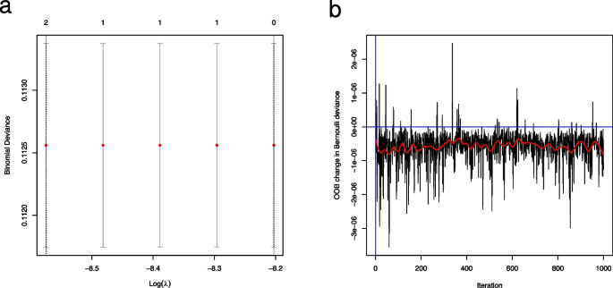
To guide the choice of hyperparameters, the primary and secondary analyses described above were implemented, and the code was tested in an approach blinded to the outcome by simulating an outcome independently from all predictors with an overall prevalence of 1%. Figure 1 includes diagnostic plots for the primary and secondary analyses. Although based upon a single simulation, the results are promising as they show that there is no tendency of the methods to overfit the data: Both methods correctly identify no relevant predictors as they should since the outcomes have been simulated independently from risk factors.
a Binomial deviance from the primary analysis of simulated outcome data. Binomial deviance as a function of the regularization parameter (on a logarithmic scale) in the LASSO regression as estimated by cross-validation. The figure contains point estimates as well as error bars signifying the standard error of the estimate. The numbers in the top of the figure denote the degrees of freedom in the model. Vertical dashed lines denote the smallest regularization estimate (leftmost line) and the smallest regularization plus one standard error. b Change in binomial deviance from secondary analysis of simulated outcome data. Out-of-bag (OOB) estimates of the change in binomial deviance as a function of the number of trees in the boosting procedure of the secondary analysis. The relationship is smoothed in the red curve, while vertical and horizontal blue lines demarcate the origin
The code was implemented in R version 4.1 using the glmnet ([38], version 4.1–4) package to fit the primary analysis and the gbm package ([34], version 2.1.8.1) for the secondary analysis. The mock analysis differed from those described above in that it was implemented on the entire data set, not stratified by sex.


Add Comment