An improved transmissibility model to detect transgenerational transmitted environmental effects | Genetics Selection Evolution

Improved transmissibility model including environmental effects

As a reminder, the transmissibility model proposed by David and Ricard [21] is as follows:

where \({y}_{i}\) is the phenotype of individual \(i\), \({\varvec{\upbeta}}\) is the vector of fixed effects with known incidence vector \({\mathbf{x}}_{\mathbf{i}}\), \({t}_{i}\) is the “global transmissible potential” of animal \(i\) that combines its different transmissible values (genetic, epigenetic, microbiote and culture [23,24,25]) with \(\mathbf{t}\sim MVN\left(0,\mathbf{M}{\sigma }_{t}^{2}\right)\), where \(\mathbf{M}\) is the matrix of transmission between individuals (transmission relationship matrix), \({\sigma }_{t}^{2}\) is the variance of the global transmissible potential, \({e}_{i}\) is the residual where \(\mathbf{e}\sim MVN\left(0,\mathbf{I}{\sigma }_{e}^{2}\right),\) and \(\mathbf{I}\) is the identity matrix. The model of transmission of the global transmissible potential is: \({t}_{i}={{\omega }_{s}t}_{si}+{{\omega }_{d}t}_{di}+{\varepsilon }_{i},\) where \({t}_{si}\) and \({t}_{di}\) are the global transmissible potential of the sire and dam of animal \(i\), and \({\omega }_{s}\) and \({\omega }_{d}\) are the unknown path coefficients of transmission from the sire and the dam, respectively, that conform to the following constraints: \(0\le {\omega }_{s}\le 1, 0\le {\omega }_{d}\le 1,\) \(0\le {\omega }_{s}+{\omega }_{d}\le 1\). \({\varepsilon }_{i}\) refers to the transmissibility sampling with \({\varvec{\upvarepsilon}}\sim N\left({\varvec{0}},\mathbf{D}{\sigma }_{t}^{2}\right),\) where \(\mathbf{D}\) is a diagonal matrix with variances of \(\varepsilon\) relative to \({\sigma }_{t}^{2}\) as components \({(\delta }_{i})\), i.e., considering no inbreeding \({\delta }_{i}=\left(1-{\omega }_{s}^{2}-{\omega }_{d}^{2}\right)\) if both parents of animal \(i\) are known, \({\delta }_{i}=\left(1-{\omega }_{d}^{2}\right)\) for animals of an unknown sire, \({\delta }_{i}=\left(1-{\omega }_{s}^{2}\right)\) for animals of an unknown dam, and 1 for animals for which both parents are unknown. Given this model of transmission, the inverse of the transmission relationship matrix can be easily obtained by the following decomposition: \({\mathbf{M}}^{{\varvec{-1}}}={\mathbf{L}}^{\mathbf{^{\prime}}}{\mathbf{D}}^{{\varvec{-1}}}\mathbf{L}\), where \(\mathbf{L}\) is a lower triangular matrix with 1s on the diagonal and the negatives of the sire and dam’s coefficients of transmission as off-diagonal entries [26, 27]. Co-variance parameters of the transmissibility model (\({\omega }_{s},{\omega }_{d}, {\sigma }_{t}^{2}, {\sigma }_{e}^{2})\) can be obtained using the ASReml software [28] and the program developed by David [20].

To improve the transmissibility model in order to account for the influence of the environment on the global transmissible potential (i.e., transgenerational transmitted environmental effect), we propose to modify the model of transmission of the global transmissible potential by including the impact of the environment in the transmissibility sampling. Thus, the transmissibility sampling is now \({\varepsilon }_{ik}={\xi }_{i}+{\theta }_{k},\) where \({\theta }_{k}\) is the random effect of environment \(k\) (\(k=1,..{n}_{E})\) experienced by animal \(i,\left( {{{\varvec{\uptheta}}}\sim MVN\left( {0,{\mathbf{I}}\sigma_{\theta }^{2} } \right)} \right),\) and \({\xi }_{i}\) is the random remaining residual of the transmissibility sampling with variance \({\sigma }_{\xi i}^{2}\). Given this decomposition, the variance of \({\varepsilon }_{ik}\) (i.e. \({\delta }_{i}{\sigma }_{t}^{2}\)) is decomposed into \(\left({\sigma }_{\xi i}^{2}+{\sigma }_{\theta }^{2}\right),\) and the covariance between transmissibility samplings of animals \(i\) and \(i{\prime}\) sharing the same environment is: \(cov\left({\varepsilon }_{ik},{\varepsilon }_{i{\prime}k}\right)={\sigma }_{\theta }^{2},\) and 0 elsewhere. \(r=\frac{{\sigma }_{\theta }^{2}}{{\sigma }_{t}^{2}}\) is defined as the proportion of total transmissibility variance explained by the environmental influence, and \(\rho =\frac{r}{1-{\omega }_{d}^{2}-{\omega }_{s}^{2}}\) as the correlation between the transmissibility samplings of animals with known parents sharing the same environment (i.e., the maximal correlation between transmissibility samplings that can be obtained). The proportion \(r\) is positive and upper bounded by \((1-{\omega }_{d}^{2}-{\omega }_{s}^{2})\) because \(\rho \le 1\). The variance of the remaining residual of transmissibility sampling for animal \(i\) is \({\sigma }_{\xi i}^{2}=\left({\delta }_{i}-r\right){\sigma }_{t}^{2}\). As a result, the co-variance matrix of \({\varvec{\varepsilon}}\) is \({\mathbf{D}}_{\mathbf{E}}{\sigma }_{t}^{2},\) where \({\mathbf{D}}_{\mathbf{E}}\) can be reorganized as a block diagonal matrix with \({n}_{E}\) blocks. Each block corresponds to one specific environment. They all have the same matrix structure of various sizes depending on the number of animals sharing the same environment \(k\): \({\delta }_{i}\) coefficients on the diagonal and coefficient \(r\) as off-diagonal entries (see Additional file 1). The transmissibility model including transmitted environmental influences is then the same as Eq. (1), but the transmissibility matrix \(\mathbf{M}\) is modified. This modified transmissibility matrix is referred to as \({\mathbf{M}}_{{\varvec{E}}}\). Once again, its inverse can be easily obtained by the decomposition: \({\mathbf{M}}_{\mathbf{E}}^{{\varvec{-1}}}=\mathbf{L}\mathbf{^{\prime}}{\mathbf{D}}_{\mathbf{E}}^{{\varvec{-1}}}\mathbf{L}\). Shared environmental effects are transmitted from one generation to another through path coefficients of transmission. A detailed description of the way to compute \({\mathbf{M}}_{\mathbf{E}}^{{\varvec{-1}}}\) is provided in Additional file 1. Thus, in the transmissibility model with environment, compared to the traditional transmissibility model, one additional parameter has to be estimated: \(r\). These parameters can be estimated with the restricted maximum likelihood method (REML) using ASReml [28] and the OWN Fortran program, freely available on the Zenodo website (https://doi.org/10.5281/zenodo.8223572), which we have developed.

Consider the special case where a group of animals experiences a particular shared environment (e.g., a stressful environment induced in an experiment) with effect \({\theta }_{0}{\sigma }_{t}\), while the other animals are each in their own environment, different from each other. In that case, information about the variance of the transmitted environmental effect leads to the difference between the average transmissibility potential of the group of animals experiencing the particular environment and the other animals. Thus, \({\sigma }_{\theta }^{2}={\theta }_{0}^{2}{\sigma }_{t}^{2}\), hence \(r={\theta }_{0}^{2}\) and \({\theta }_{0}<\sqrt{(1-{\omega }_{d}^{2}-{\omega }_{s}^{2})}\). The reorganized \({\mathbf{D}}_{\mathbf{E}}\) matrix has only one block, as previously defined, and the remaining matrix is diagonal with \({\delta }_{i}\) terms.

Simulation study

The aim of the simulation study was to evaluate the performances of the transmissibility model with environment so as to detect and quantify transgenerational transmitted environmental effects and not to confuse them with non-transmissible environmental effects. Indeed, on the one hand, the effect \({\theta }_{k}\) of environment \(k\) may be transmissible across generations; in which case it has an effect on the transmissible potential \({t}_{i}\) of animal \(i\) experiencing environment \(k\) as described above. On the other hand, the effect of the environment may not be transmissible but nonetheless it may have an impact on the phenotype of animal \(i\). In this case, the environmental effect can be modeled as a fixed effect of the mixed model used to simulate the phenotype. These two situations were investigated in the simulations.

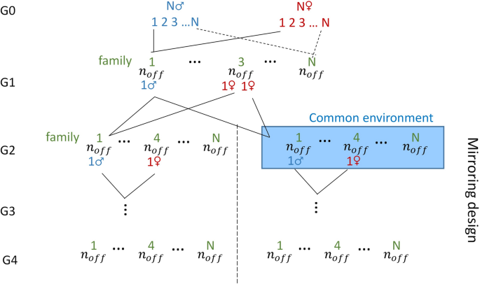
A population that mimics a mirrored experimental design proposed by Leroux et al. [29] was simulated for the purpose of testing the transmission of environmental effects across generations (Fig. 1). The population consisted of \(N\) couples of founders (\(N\) families: G0) that gave birth to \({n}_{off}\) offspring each (G1). One male of each family in G1 was then mated to two sisters of another family that then gave birth to two groups of \({n}_{off}\) offspring (\(2N{n}_{off}\) animals in G2). Half of the groups (one for each family; \(N{n}_{off}\) animals) was then considered as experiencing the same particular environment, for example a stressful environment, (from this point on, the descendants of the two groups are qualified as belonging to two different lines: \(E+,E-\)). Three generations were then produced for each line with exact parallel pedigrees via mirrored single-pair matings at each generation.

Simulated population in the mirroring design. \(N\) is the number of pairs of male and female founders; \({n}_{off}\) is the number of offspring per pair

Phenotypes were simulated for all animals, and different scenarios for modeling the impact of the environment were considered. In Scenario 1, the environment has an impact on the phenotype but is not vertically transmitted. It was simulated by adding a constant to the phenotype of animals that experienced the stressful environment; \({y}_{i}={\mathbf{x}}_{\mathbf{i}}{\varvec{\upbeta}}+{\theta }_{i}+{t}_{i}+{e}_{i}\), where \({\theta }_{i}=\sqrt{r}{\sigma }_{t}\) if animal \(i\) is in the particular environment and \({\theta }_{i}=\) 0 elsewhere, and \({t}_{i}\) is modeled as in the “classical” transmissibility model. In Scenario 2, the environment has an impact on the transmissible potential (i.e., it is a transmitted environmental effect). This impact was modeled by adding a constant to the transmissible potentials of animals experiencing the stressful environment, i.e., \({t}_{i}={{\omega }_{s}t}_{si}+{{\omega }_{d}t}_{di}+{\theta }_{i}+{\xi }_{i}\), where \({\theta }_{i}=\sqrt{r}{\sigma }_{t}\) if animal \(i\) is in the particular environment and \({\theta }_{i}=\) 0 elsewhere, and \({\varvec{\upxi}}\) were independently distributed with variance equal to \(\left({\delta }_{i}-r\right){\sigma }_{t}^{2}\) for animals that experienced the particular environment, and \({\delta }_{i}{\sigma }_{t}^{2}\) elsewhere.

The same four sets of parameters were used in the two scenarios (Table 1), the difference between scenarios being how the phenotypes were simulated (transmitted or not transmitted environmental effect). Values of \(r\) were chosen in order to correspond to a wide range of values for \(\rho\) (from 0.30 to 0.70), the maximal correlation that can be obtained between transmissibility samplings of animals sharing the same environment when the environmental effect is transgenerationally transmitted.

The transmissibility model and the transmissibility model with environment were applied to the simulated data of the different scenarios (100 replicates each and for each set of parameters). The environment (cross-classified variable equal to 1 if animals experience the particular environment, 0 elsewhere) was included as a fixed effect in both models. The null hypothesis of “no transmitted environmental effect” (i.e., \(r=0\)) was tested by comparing the two models using a likelihood ratio test (LRT). Because the test corresponds to a test at the boundary of the parameter space of \(r\), the asymptotic distribution of the LRT is a 50:50 mixture, \({\chi }_{0}^{2}\) and \({\chi }_{1}^{2}\) [30]. The null hypothesis was then rejected at the \(\alpha\)-risk of \(5\%\) if the LRT was greater than 2.706. The transgenerational effect of the environment was also assessed, as previously done in the literature, by comparing the phenotypic performance of the two lines in the last generation [29, 31, 32]. The difference in the average phenotype of the two lines in the last generation was tested using a paired T-test at the \(\alpha\)-risk of 5%. Using these different scenarios and these two models of estimation, our aim was (i) to estimate the realized type I error of the LRT and the paired T-tests when there is an environmental effect but that is not transmissible (Scenario 1); and (ii) to estimate the power of the LRT and the paired T-tests to detect the transmitted environmental effects of different importance and to illustrate the capacity of the transmissibility model with environment to correctly estimate parameters (Scenario 2). For all the simulations, \(N=20, {n}_{off}=10,\) leading to 1840 animals in the pedigree. The residual variance was fixed to 10 and the transmissibility variance to 5 in all scenarios.

To illustrate the ability of the transmissibility model with environment to correctly estimate parameters in any population with many different environments, we also performed an additional simulation considering the same population structure as used in David and Ricard [21], 15 different particular environments and the simulation parameters of set 1 (see Additional file 2 for details).